Food Security Metrics in South Sudan: Comparing the gold standard with a pile of dried beans
Hayley Umayam - Statistics for International Relations Research II
Introduction
Background
Recent estimates suggest that over half the population of South Sudan is facing severe acute food insecurity (South Sudan IPC Technical Working Group 2020). By the summer of 2021, this number is projected to increase to 60% of the population (7.24 million people) who will fall under ‘crisis’, ‘emergency’ or ‘catastrophe’ classifications of food insecurity, including 31,000 individuals likely to be facing conditions of famine (South Sudan IPC Technical Working Group 2020). While this phenomenon is clearly a grave, real world problem warranting political attention and resolution (Gustafsson and Hagström 2018), my experiences close to the processes that produced these classifications compels me to look at the situation more critically.
The Integrated Food Security Phase Classification’s (IPC) five-phase scale, with phases distinguished by thresholds of food consumption, child malnutrition, or related mortality, has become “the global standard” for classifying situations of acute food insecurity (The IPC Famine Factsheet 2020). With the tagline, “Evidence and Standards for Better Food Security and Nutrition Decisions,” IPC products are highly influential in humanitarian responses in contexts such as South Sudan, where they are used to pinpoint geographic areas of need. The numbers presented in the IPC’s reports are cited in project proposals and appeals for funding to international donors as large and small humanitarian organizations design needs-based responses aimed at reaching “the most food insecure.” Color-coded IPC maps are projected at emergency response coordination meetings, guiding discussions about which counties should be prioritized with the limited resources available. Even news articles and security updates are peppered with the numbers describing current and projected food security.
The popularity of IPC metrics is just one example of the range of approaches to describe levels of food related needs. Beyond assessments such as early warning and nutrition surveillance systems that seek to identify populations in need, there are reporting processes such as through which humanitarian organizations will account for their response to (identified) need, as well as monitoring processes which seek to further reconcile need with responses. So important are these processes, that entire units within humanitarian organizations are dedicated to the collection of such information or such tasks are outsourced to service providers. However, despite the increasing range and usage of processes for describing food security need, the humanitarian system continues to struggle to respond to and prevent food security crises in South Sudan. We would expect that more tools and processes to translate the ‘needs’ of affected populations into actionable data would lead to better informed decisions about where to direct food aid. However, numerous studies continue to note a disconnect in understandings of need between localities, humanitarian actors and policy makers. Why is there a disconnect between what affected populations want and what they receive even though humanitarian service providers have a variety of processes for measuring levels of need?
Research Question & Hypothesis
I suspect that the reason studies continue to note differences in how affected populations and humanitarian actors understand levels of food need relates to the processes by which humanitarians solicit, interpret, and aggregate information. For instance, the Food Consumption Score (FCS) attempts to present a standardized approximation of a household’s level of need upon which decisions of providing food interventions are made. FCS information is a critical component for determining an IPC classification for a given location, a determination that has implications for subsequent humanitarian assistance. But do the needs of affected populations as identified by popular metrics of humanitarian agencies like the FCS align with what affected populations say they need?
In 2017-2019, a team of researchers put this to the test, by collecting information not only on the FCS of households in South Sudan, but also asking them how they would prioritize resources in their own community if given the chance. This was done through a piling exercise, during which respondents demonstrated the amount of resources they would dedicate to a different area (education, infrastructure, food aid, etc) if they could decide, by placing different numbers of dried beans on different representations of the areas. We can understand this piling exercise as an alternative way to understand need, with the assumption that participants would allocate more resources to areas they feel their community needs the most. We simplify this inquiry into prioritizing direct food aid or any other area. This allows us to as the following research question: What does a household’s FCS tell us about the odds that they would chose to prioritize direct food assistance if given the chance? Put differently, does the gold standard (FCS) tell us information that is any different than a pile of beans could tell us in terms of which households are in need?
If FCS aligned with the priorities of affected populations, we would expect that households with lower FCS would prioritize direct food aid over other types of interventions. Misalignment could indicate that people’s needs and priorities are more complex than a metric like the FCS can capture and reflect.
- Null Hypothesis: FCS match how households would prioritize
resources.
- Observable implication: As FCS decrease, households prioritize direct food aid over other types of assistance.
- Alternative Hypothesis: FCS do not match how households would
prioritize resources.
- Observable implication: As FCS decrease, households prioritize other types of assistance over direct food aid.
TLDR: What did we learn in this exploration?
Using a binomial logit regression, we find support for the null hypothesis. In general, it does appear that the odds a household would prefer direct food aid over other types of food assistant are higher in households with lower FCS. This trend generally holds even when we control for basic demographic features and the person who controls how resources in a household are used. However, results are distinct enough to support calls for understanding gender roles in relation to household food security.
Since this preliminary analysis does not seem to support our hypothesis, does this mean the FCS is perfectly aligned with community preferences? Not necessarily. The findings here can not be interpreted without consideration of the limitations of the data from which they are drawn and of the model specifications used to explore our hypothesis. Nonetheless, this study provides a helpful starting point from which subsequent inquiries related to food security metrics may be built.
Data
For this inquiry, I draw on an existing data set of household-level survey data compiled by myself and my colleagues (see Annex). The raw data set contains 1,552 observations collected in South Sudan between March-November 2019. This survey was originally meant to supplement qualitative monitoring exercises conducted at the sites of various humanitarian interventions across the country by providing community perceptions in relation to humanitarian programming in general.
This survey was not designed to be representative of a given geographic area or of the direct beneficiaries of a given humanitarian intervention. Rather, this survey selected households in the general population residing within the “catchment area” of specific humanitarian programs being monitored. It is important to note that in spite of rhetoric about reaching the most remote populations with the greatest need, most humanitarian interventions are clustered around a few established ‘hubs’. As monitoring took place where the interventions were conducted, this sample reflects this clustering around services. It is therefore recognized that this data may therefore be biased towards those with more access to, knowledge of, and potentially participation in humanitarian programming, while it under-represents those in more remote locations. Any investigation is exploratory; any insights are limited as suggestions of wider trends. To make this data usable, it was necessary to clean the data set. The majority of cleaning related to enumerator error and measurement error. These processes will be further explored in subsequent works. The final, cleaned data set contains 1,450 observations.
Variables of Interest
This survey was intended to explore community-level perceptions relevant to humanitarian programming. It contained multiple modules, but only those related to demographics, food security, and the piling exercise are utilized for the present hypothesis.
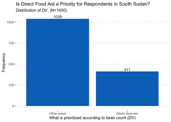
The dependent variable of interest is a binary, categorical variable
with the value of 1 if a respondent piled more dried beans on the
category of “direct food aid” than they did on any other category, and a
value of 0 if otherwise. Based on frequency, we see that the majority of
respondents prioritized areas other than direct food aid.
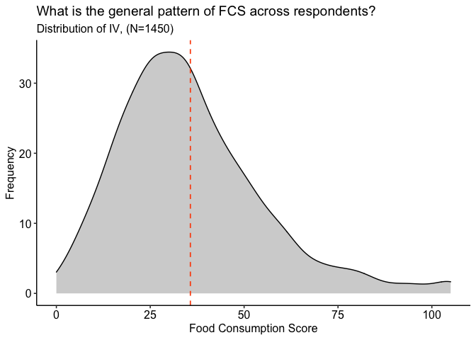
The independent variable of interest is the Food Consumption Score (FCS) of a household. This is a continuous, numeric variable based on industry best practices (https://inddex.nutrition.tufts.edu/data4diets/indicator/household-dietary-diversity-score-hdds). As shown below, the distribution of FCS among respondents is right-tailed, with most respondents having a score of less than 50 (the median). The dotted red line falls on the mean, which is roughly 36.
Control variables
The choice of potential control variables was guided by the knowledge of the limitations of this data set. Given the exploratory nature of this hypothesis testing, the author was weary to include too many controls. For instance, while there are important differences in geography to account for, many administrative boundaries in South Sudan are currently contested. It was therefore deemed inappropriate to control for this using variables available in the data set, as existing variables would only support politically-motivated distinctions that may or may not align with more pertinent characteristics of a population in that particular area. It was also deemed inappropriate to explore household income or other economic factors at this point, with the assumption that these factors would co-vary with food consumption.
Current transformations brought about by conflict and political-economic developments are directly impacting gender roles and behaviors throughout society. Nonetheless, in many areas of South Sudan, food-related tasks are gendered, with women bearing primary responsibility for much of a household’s daily food needs. Further, humanitarian assistance can sometimes reinforce existing gender roles (Mulukwat 2017). Therefore it is important to take gender and decision making into account when considering matters of food security and household resources.
Existing literature also suggests that levels of education have an effect on household food security, but that these effects are context dependent (Mutisya et al 2016).
Thus, three control variables are included: 1) the gender of the respondent; 2) the gender of the household member who decides how resources in the home will be used; and 3) education level. We also explore an interaction between gender and education level.
Methods & Models
Given the nature of our DV of interest (categorical), and our RQ that seeks to calculate estimates for this data, a binomial logistic regression was deemed the most appropriate. Logits are also useful since they can be transformed into odds ratios, which is perhaps easier to interpret (Hollway Lecture 5 - Binary). It was not deemed appropriate to transform any variables of interest through logging or squaring, since many are categorical and the numeric variables are well contained. The aforementioned limitations of the data set call for some restraint when it comes to model specification. We test a simple model (Model 1) that includes only our DV & IV, a model with all our control variables (Model 2), and a model with all control variables plus an interaction term (Model 3).
Preliminary Findings support the null
We can compare the log-odds of our parameters across models as an initial hypothesis test. This allows us to understand the probability of prioritizing direct food aid (our DV) as a function of an intercept, IV, our control variables, and an error term. The results table showing log odds can be found in the Annex.
In this preliminary analysis, the coefficient of FCS (the IV) is significant (differentiable from zero) and it is negative, suggesting that an increase in FCS, decreases the odds of prioritizing direct food aid. However, we note that the beta value of the IV log-odds is quite small. More interestingly, this “sign-ificance” (Hollway Lecture 5 - Binary) of the IV remains the same across all 3 models. Regardless of the controls used or presence of an interaction term, holding all else constant, the IV remains significant and negative.
Therefore in general, these models seem to support the idea that FCS is a good metric (in the sense that it seems to align with areas that individuals would themselves prioritize).
However, this general indication does not allow us to chose between models. We can run our regression models using the sjPlot function in R to understand the respective odds ratios of our parameters, which is easier to interpret.
| Model 1: simple | Model 2: with controls | Model 3: interaction | |||||||
|---|---|---|---|---|---|---|---|---|---|
| Predictors | Odds Ratios | CI | p | Odds Ratios | CI | p | Odds Ratios | CI | p |
| (Intercept) | 0.64 | 0.50 – 0.82 | <0.001 | 0.47 | 0.33 – 0.66 | <0.001 | 0.37 | 0.24 – 0.55 | <0.001 |
| IV.continuous | 0.99 | 0.98 – 0.99 | <0.001 | 0.99 | 0.98 – 1.00 | 0.001 | 0.99 | 0.98 – 1.00 | 0.003 |
| d\_sex \[Female\] | 1.46 | 1.10 – 1.93 | 0.008 | 1.97 | 1.37 – 2.87 | <0.001 | |||
| d\_education | 0.95 | 0.92 – 0.97 | <0.001 | 0.98 | 0.95 – 1.02 | 0.279 | |||
| hh\_moneyuse \[Female HoHH\] | 1.20 | 0.91 – 1.59 | 0.200 | 1.18 | 0.89 – 1.56 | 0.262 | |||
| hh\_moneyuse \[Both\] | 1.64 | 1.20 – 2.24 | 0.002 | 1.68 | 1.23 – 2.29 | 0.001 | |||
| d\_sex \[Female\] \* d\_education | 0.93 | 0.89 – 0.98 | 0.010 | ||||||
| Observations | 1450 | 1450 | 1450 | ||||||
| R2 Tjur | 0.013 | 0.044 | 0.048 | ||||||
Across all three models, the results suggest that holding all over parameters constant, as FCS increases (by one unit) the odds of prioritizing direct food aid decrease by 0.99 (or 169% if we exponentiate). This finding is statistically significant.
When looking at the effect of gender, Model 2 indicates that being a female respondent increases the odds of prioritizing direct food aid by 1.46 (or roughly 330% if we exponentiate), as compared to male respondents, holding all other parameters constant. This relationship is consistent in its direction and significance across Model 2 and 3.
Education appears to have a positive effect on the odds of prioritizing direct food aid, but it is only statistically significant in Model 2. However, the interaction term between the gender of a respondent and their level of education is shown to be statistically significant in Model 3.
However, we should not get too carried away with our substantive interpretations of either log odds or odds ratios. For instance, Mood (2010) would suggest that we should pay attention to predicted probabilities, marginal effects, and average marginal effects. Norton and Dowd (2018) reiterate this, and emphasize that AME are preferable to odds ratios due to how odds ratios are computed. Therefore, once a model is selected, we will put more stock in the results of these other indicators (see: Results)
Selecting a model
We have three models and each include statistically significant results, but that doesn’t automatically mean they are all of equal utility. Ideally, we would select a model that, in comparison to others, appears to fit our data best. We can do this by looking at Likelihood Ratios, AIC, and the ROC.
## Likelihood ratio test
##
## Model 1: DV.binary ~ IV.continuous
## Model 2: DV.binary ~ IV.continuous + d_sex + d_education + hh_moneyuse
## Model 3: DV.binary ~ IV.continuous + d_sex + d_education + hh_moneyuse +
##     d_sex * d_education
##   #Df  LogLik Df   Chisq Pr(>Chisq)
## 1   2 -854.58
## 2   6 -832.13  4 44.9060  4.159e-09 ***
## 3   7 -828.75  1  6.7437   0.009408 **
## ---
## Signif. codes:  0 '***' 0.001 '**' 0.01 '*' 0.05 '.' 0.1 ' ' 1
The Likelihood Ratio Test compares the likelihood scores of the three models to determine if the difference between the three is statistically significant, by testing if the predictors are jointly significant. Based on the output of this LR test, which gives us a p-value less than 0.05 for Models 2 and 3, we can reject the null hypothesis that the smaller model (Model 1) is true. Therefore, we would chose Model 2 or Model 3, as there evidence against the reduced model alternative.
We can also revisit our regression results, this time including AIC for comparison, which is appropriate since we are training the models on the exact same data.
| DV.binary | DV.binary | |||||
|---|---|---|---|---|---|---|
| Predictors | Odds Ratios | CI | p | Odds Ratios | CI | p |
| (Intercept) | 0.47 | 0.33 – 0.66 | <0.001 | 0.37 | 0.24 – 0.55 | <0.001 |
| IV.continuous | 0.99 | 0.98 – 1.00 | 0.001 | 0.99 | 0.98 – 1.00 | 0.003 |
| d\_sex \[Female\] | 1.46 | 1.10 – 1.93 | 0.008 | 1.97 | 1.37 – 2.87 | <0.001 |
| d\_education | 0.95 | 0.92 – 0.97 | <0.001 | 0.98 | 0.95 – 1.02 | 0.279 |
| hh\_moneyuse \[Female HoHH\] | 1.20 | 0.91 – 1.59 | 0.200 | 1.18 | 0.89 – 1.56 | 0.262 |
| hh\_moneyuse \[Both\] | 1.64 | 1.20 – 2.24 | 0.002 | 1.68 | 1.23 – 2.29 | 0.001 |
| d\_sex \[Female\] \* d\_education | 0.93 | 0.89 – 0.98 | 0.010 | |||
| Observations | 1450 | 1450 | ||||
| AIC | 1676.252 | 1671.508 | ||||
| log-Likelihood | -832.126 | -828.754 | ||||
In the results table above, we see that Model 3 has a slightly lower AIC value than Model 2, suggesting we select the former. As once final check, we will also consider the accuracy of the models by examining the Receiver Operating Characteristic (ROC) curve plots.
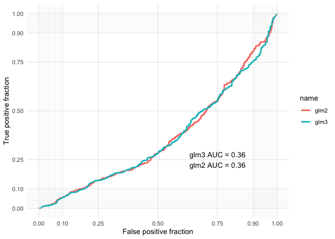
The Area under the Curve (AUC) values tell us two key things. First, that both Model 2 (glm2) and Model 3 (glm3) perform the same in terms of the accuracy of classification. However, more importantly, neither of these models seem to give us much confidence in the accuracy of their classifications. At 0.64, these models are just shy of a total failure (Hollway Lecture 5 - Binary).
Together, the LR test and AIC values suggest that we should use Model 3 to explore our hypothesis, but our AUROC values remind us to exercise constraint with the findings, given that our models may not be as accurate as we might like.
Results
Bearing in mind the limitations of our selected model, we now seek to explore support for our hypothesis through predicted probabilities and marginal effects.
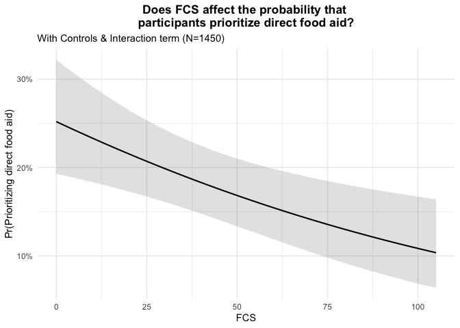
Indeed, holding all else equal, the predicted probability graph for Model 3 indicates a negative association between the probability an individual prioritizes direct food aid and their food consumption score. In other words, the higher an individuals food consumption score, the less probable they are to prioritize direct food aid.
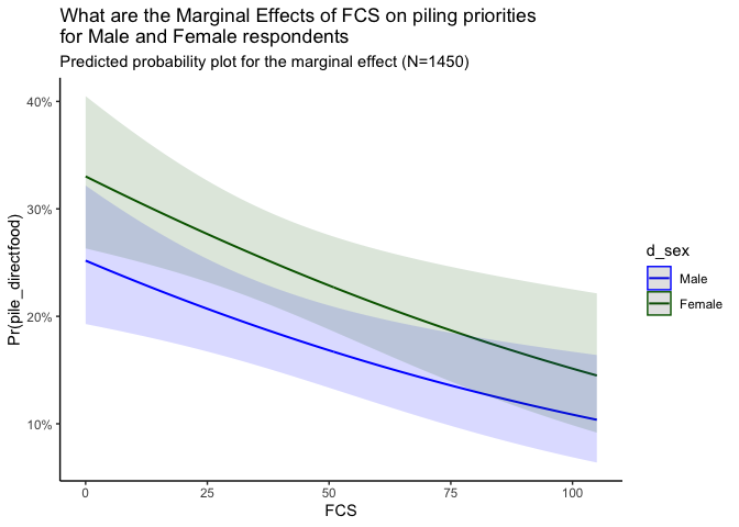
Based on the plot above, which assumes all other variables are held constant, we see a familiar pattern in that those with higher FCS have a lower probability of prioritizing direct food aid. This trend holds for both male and female respondents alike. However, given the higher intercept of female respondents and otherwise parallel lines, it appears that the odds of a female respondent prioritizing direct food aid over other forms of assistance are higher than that of male respondents, regardless of their FCS.
##         factor     AME     SE       z      p   lower   upper
##    d_sexFemale  0.0806 0.0258  3.1211 0.0018  0.0300  0.1312
##  IV.continuous -0.0020 0.0006 -3.0485 0.0023 -0.0032 -0.0007
The table showing average marginal effects (AME) supports this as well. The sign of the AME for d_sex is positive and statistically significant; and for FCS it is negative and significant. This can be interpreted as the average marginal effect of an additional unit of FCS is a decrease of 0.0021 on the predicted probability (a decrease by 0.2 percentage points on average) and the predicted probability of prioritizing direct food aid for female respondents is 0.0718 (an increase of 7 percentage points on average) more on average than for male respondents.
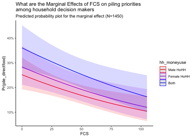
The plot above, again assuming all other variables are held constant, reveals a similar trend, but adds another layer. In households where both spouses decide how resources will be used, the odds that they will prioritize direct food aid over other types of assistance are higher than that of a female headed household or a male headed household. This finding might give some support to notions of changing gender roles and their effect on household food security, as suggested by the literature cited above.
Conclusion
This study has used binomial logit regressions to explore how well a commonly used food security metric aligns with the priorities of affected populations in South Sudan. In general, findings indicate that households with lower food consumption scores have higher odds of prioritizing direct food aid than households with higher food consumption scores. While this preliminary analysis does not seem to support our hypothesis, the results should be understood as exploratory, given some of the shortcomings in the accuracy of the selected models. Nonetheless, these preliminary findings can be used to inform subsequent inquiries such as:
- Repeating the exploration outlined above, with data that is more geographically representative
- Repeating the exploration outlined above, but with a non-binary categorical DV or by restructuring the nature of the existing binary DV (i.e. grouping any food-related area such as direct food aid and agricultural support together)
- Repeating the exploration outlined above with other common metrics of food security (such as dietary diversity scores) as a IV
- Exploring more model specifications that yield higher accuracy in their classification. This might include controls for age.
- Exploring how priorities (piling exercise) are effected by notions of social cohesion or other forms of humanitarian programming happening in that area (this data is currently available in the existing data set, but will require significant “wrangling”)
- Comparing results with other studies exploring changes in gender roles
- Exploring the data generating processes that produce the survey observations utilized for this and other surveys to better understand how food security metrics are understood by a variety of interlocutors.
References
Gustafsson, K,, & Hagström, L (2018). “What Is the Point? Teaching Graduate Students How to Construct Political Science Research Puzzles.” European Political Science 17, no. 634–48. https://doi.org/10.1057/s41304-017-0130-y.
Mulukwat, K. (2017). “Gender Norms, Conflict, and Aid - briefing note.” Conflict Sensitivity Resource Facility. https://www.csrf-southsudan.org/repository/gender-norms-conflict-aid-briefing-note/
Mood, C. (2010) Logistic Regression: Why We Cannot Do What We Think We Can Do, and What We Can Do About It, European Sociological Review, 26(1), 67–82, https://doi.org/10.1093/esr/jcp006
Mutisya, M., Ngware, M.W., Kabiru, C.W. et al. (2016). “The effect of education on household food security in two informal urban settlements in Kenya: a longitudinal analysis.” Food Sec. 8, 743–756 https://doi.org/10.1007/s12571-016-0589-3
Norton, E. C., & Dowd, B. E. (2018). Log Odds and the Interpretation of Logit Models. Health services research, 53(2), 859–878. https://doi.org/10.1111/1475-6773.12712
“The IPC Famine Factsheet.” Factsheet. Integrated Food Security Phase Classification, 2020. https://reliefweb.int/report/world/ipc-famine-factsheet-updated-december-2020.
R Packages
Fox J, Weisberg S (2019). An R Companion to Applied Regression, Third edition. Sage, Thousand Oaks CA. https://socialsciences.mcmaster.ca/jfox/Books/Companion/.
John, Christopher (2020) MLeval: Machine Learning Model Evaluation. https://cran.r-project.org/web/packages/MLeval/index.html
Kassambara, Alboukadel (2020). ggpubr: ‘ggplot2’ Based Publication Ready Plots. R package version 0.4.0, https://cran.r-project.org/web/packages/ggpubr/index.html.
Leeper TJ (2021). margins: Marginal Effects for Model Objects. R package version 0.3.26.https://cran.r-project.org/web/packages/margins/citation.html
Lüdecke D (2021). sjPlot: Data Visualization for Statistics in Social Science. R package version 2.8.8, https://CRAN.R-project.org/package=sjPlot.
Revelle W (2021). psych: Procedures for Psychological, Psychometric, and Personality Research. Northwestern University, Evanston, Illinois. R package version 2.1.3, https://CRAN.R-project.org/package=psych.
Rich, Benjamin (2021). table1: Table of Descriptive Statistics in HTML. https://cran.r-project.org/package=table1
Sachs, Michael C. (2017). plotROC: A Tool for Plotting ROC Curves. Journal of Statistical Software, Code Snippets, 79(2), 1-19.doi:10.18637/jss.v079.c02
Wickham H, Averick M, Bryan J, Chang W, McGowan LD, François R, Grolemund G, Hayes A, Henry L, Hester J, Kuhn M, Pedersen TL, Miller E, Bache SM, Müller K, Ooms J, Robinson D, Seidel DP, Spinu V, Takahashi K, Vaughan D, Wilke C, Woo K, Yutani H (2019). “Welcome to the tidyverse.” Journal of Open Source Software, 4(43), 1686. doi: 10.21105/joss.01686.
Annex
Additional notes on the data
The survey from which this data is drawn was collectively designed and managed by the ELFSS team from 2017-2020, which included Philip Taban, Lokiri Moses, Brendan Tuttle, Eero Wahlstedt, Hayley Umayam, Angelina Gon, Holly Moses, Nyama Williams, Kur Kur, and others. Data collection was conducted by numerous enumerators, without whom this work would not be possible.
Model Comparison using Log Odds
#comparing models with log-odds
| Model 1: simple | Model 2: with controls | Model 3: interaction | |||||||
|---|---|---|---|---|---|---|---|---|---|
| Predictors | Log-Odds | CI | p | Log-Odds | CI | p | Log-Odds | CI | p |
| (Intercept) | -0.44 | -0.69 – -0.20 | <0.001 | -0.76 | -1.11 – -0.41 | <0.001 | -1.00 | -1.41 – -0.60 | <0.001 |
| IV.continuous | -0.01 | -0.02 – -0.01 | <0.001 | -0.01 | -0.02 – -0.00 | 0.001 | -0.01 | -0.02 – -0.00 | 0.003 |
| d\_sex \[Female\] | 0.38 | 0.10 – 0.66 | 0.008 | 0.68 | 0.32 – 1.05 | <0.001 | |||
| d\_education | -0.05 | -0.08 – -0.03 | <0.001 | -0.02 | -0.06 – 0.02 | 0.279 | |||
| hh\_moneyuse \[Female HoHH\] | 0.18 | -0.10 – 0.46 | 0.200 | 0.16 | -0.12 – 0.44 | 0.262 | |||
| hh\_moneyuse \[Both\] | 0.50 | 0.19 – 0.81 | 0.002 | 0.52 | 0.20 – 0.83 | 0.001 | |||
| d\_sex \[Female\] \* d\_education | -0.07 | -0.12 – -0.02 | 0.010 | ||||||
| Observations | 1450 | 1450 | 1450 | ||||||
| R2 Tjur | 0.013 | 0.044 | 0.048 | ||||||
Co-Director
Global Governance Centre
Professor
International Relations and Political Science
President
Global Governance Research Centre Consortium
International institutions and political networks.