Marine Gauthier
Data: REDD.dta This dataset and its indexes have been constructed on the basis of the data made available by the International Database on REDD+ projects and programs. Simonet G., Agrawal A., Bénédet F., Cromberg M., de Perthuis C., Haggard D., Jansen N., Karsenty A., Liang W., Newton P., Sales A-M, Schaap B., Seyller C., Vaillant G., (2018) ID-RECCO, International Database on REDD+ projects and programs, linking Economic, Carbon and Communities data. version 3.0. http://www.reddprojectsdatabase.org
1. Introduction
Over the last twelve years, International Organizations have increasingly targeted the forests of the Global South as a way to mitigate climate change. Tropical rainforests are seen as a stabilizing force for the climate to regulate ecosystems, protect biodiversity and absorb carbon emissions, but also as a threat for the climate, with deforestation and land-use change accounting for nearly 20% of all greenhouse gas emissions — more than the world’s entire transport sector – adding to the loss of their removal capacity (Karsenty, 2004). This calculation has strategically shifted the focus of climate mitigation policies away from northern industrial drivers of carbon emissions to the global need to save the southern rainforests through both the carbon market-based financial incentives and governance support programmes. Initially excluded from the Kyoto Protocol, tropical deforestation is now a viable object of climate governance, constructed through the mobilization of expert knowledge on carbon cycle and carbon accounting, on global land cover change and remote monitoring technologies (Boyd, 2010).
Halting deforestation has become a priority for UN programs, the World Bank and bilateral cooperation between States. A product of the trans-nationalization of global environmental politics, the REDD+ (Reducing Emissions from Deforestation and Degradation of Forests) is a mechanism developed by Parties to the United Nations Framework Convention on Climate Change (UNFCCC) in 2010. It represents the political translation of the upsurge of tropical rainforests on the post-Kyoto climate negotiations scene. By creating a financial value for the carbon stored in forests and offering incentives for southern countries to reduce emissions from forested lands and invest in low-carbon paths to sustainable development, it is a market-based solution to deforestation, and ultimately to climate change. It revolves around the idea of financially incentivizing rainforest countries to avoid deforestation by engaging with northern countries and investors playing the role of REDD+ funders. The funds are to be channeled through three main ways: (1) more “business as usual” development grants programmes offering support through policy and measures to improve governance capacities at the national level (2) performance-based payments and payment through the carbon-market targeting specific REDD+ projects, either small-scale or “integrated” in one country’s region. REDD+ “trade-not-aid” rhetoric has been promoted in many reports, mainly commissioned by major REDD+ funders such as Norway (Angelsen and al., 2009), suggesting that it could help southern countries become more autonomous from development aid.
REDD+ aims at reconciling forest conservation, social development and market-based logic, three usual antagonists, hence answering the tripartite dilemma of sustainable development, as market-logics and foreign direct investments are more often correlated to depletion of natural resources and incomes (Long, Stretesky, Lynch, 2017).
The underlying question below REDD+ logic revolves under the drivers of deforestation: what drives deforestation, and how to counter these drivers? The pendent question I would like to ask here is : “what drives deforestation reduction?”. No assessment so far of both of REDD+ axis (development support or project-based support) have been assessed and compared. Outline research question and main hypotheses (≤3)
This dataset will be used to examine the covariates of the evolution of the deforestation rate between 2010 and 2015 in REDD+ countries.
What conditions pertaining to either project-based REDD+ support or the evolution of development indicators can explain the evolution of the deforestation rate in countries engaged in Reducing their emissions from deforestation and degradation of forests?
The null hypothesis are : 1/ the more advanced REDD+ project-based support is, the more deforestation rate would decrease 2/ as the governance indicators increase, the deforestation rate would decrease 3/ A combination of both REDD+ project-based support and governance indicators increase would have a higher correlation with a decrease of deforestation rate
2. Data
This dataset has been created for the sake of this research on the basis of the data made available by the ID-RECCO, a project from the CIFOR (Bogor, Indonesia), Climate Economics Chair (Paris-Dauphine university, France), CIRAD (Montpellier, France) and IFRI (University of Michigan, United States).
The ID-RECCO database offers data on REDD+ countries and projects through a series of datasets. The dataset I created for this assignment combines two of the datasets offered by the ID-RECCO, on the REDD+ countries and one of the REDD+ projects registered in the various countries. Indexes have been created from different variables in order to offer a perspective on the evolution of the deforestation rate over the period between 2010 and 2015.
The unit of analysis is the States involved in REDD+, receiving REDD+ funds and targetted by the program to reduce their deforestation rate.
library(readxl)
library(haven)
library(tidyverse)
library(dplyr)
library(ggcorrplot)
library(qqplotr)
library(ggpubr)
library(corrplot)
library(ggcorrplot)
library(rmarkdown)
library(sjPlot)
library(sjmisc)
library(sjlabelled)
library(haven)
library(ggplot2)
library(tidyverse)
library(broom)
library(dplyr)
library(stargazer)
library(ggplot2)
library(sandwich)
library(sjPlot)
library(ggfortify)
library(ggcorrplot)
library(car)
library(margins)
library(plotROC)
library(nnet)
library(plot3logit)
library(forcats)
library (sjmisc)
library(survey)
library(table1)
library(rpart)
library(lmtest)
library(forecast)
library(lindia)
library(car)
library (outliers)
library(olsrr)
library(lawstat)
library(performance)
library(see)
library(DMwR)
library(gridExtra)
library(mice)
library(randomForest)
Here is the dataset:
#setwd("~/Dropbox/PhD/SPRING 2020/Stats II/Final")
REDD <- read_excel("REDD.xlsx")
data("REDD", package = "pscl")
REDD <- REDD %>%
  mutate(continent = as_factor(continent),
         fund = as_factor(fund))
REDD$fpic <- REDD$fpic...7
REDD$part <- REDD$participation...8
REDD$def <- REDD$deforest_10_15
REDD$Gov <-  REDD$Goveffectiveness
summary(REDD)
deforest_10_15 country_name continent Min. :-4.340280 Length:74
Africa :32
1st Qu.:-0.124908 Class :character Asia :16
Median :-0.006446 Mode :character Latin :22
Mean :-0.082382 Oceania: 4
3rd Qu.: 0.015512
Max. : 3.756481
fund rpp projects
Amazon Fund : 1 Min. :0.000 Min. : 0.000
Congo Basin Forest Fund;FCPF;UNREDD: 3 1st Qu.:0.000 1st Qu.: 1.000
FCPF : 4 Median :1.000 Median : 3.000
FCPF;UNREDD :39 Mean :1.932 Mean : 6.311
No :11 3rd Qu.:4.000 3rd Qu.: 6.750
UNREDD :16 Max. :6.000 Max. :59.000
fpic...7 participation...8 IDH GDPhab
Min. :0.00000 Min. :0.0000 Min. :-0.02600 Min. :0.6849
1st Qu.:0.00000 1st Qu.:0.7143 1st Qu.: 0.00900 1st Qu.:1.0183
Median :0.05556 Median :0.8000 Median : 0.01500 Median :1.0866
Mean :0.20109 Mean :0.7962 Mean : 0.01679 Mean :1.0869
3rd Qu.:0.33333 3rd Qu.:1.0000 3rd Qu.: 0.02300 3rd Qu.:1.1571
Max. :1.00000 Max. :1.0000 Max. : 0.09700 Max. :1.3069
NA’s :17 NA’s :17 NA’s :1
Goveffectiveness Corrupt idh_2011 idh_2015
Min. :-0.810000 Min. :-1.92000 Length:74 Min. :0.3520
1st Qu.:-0.135000 1st Qu.:-0.48000 Class :character 1st Qu.:0.4950
Median : 0.010000 Median : 0.09000 Mode :character Median :0.5890
Mean : 0.009459 Mean : 0.02329 Mean :0.6011
3rd Qu.: 0.150000 3rd Qu.: 0.48000 3rd Qu.:0.7265
Max. : 0.640000 Max. : 1.71000 Max. :0.8470
NA’s :1
gdp_hab_2012 gdp_hab_2016 deforestation_rate_2010 Min. : 236.0
Min. : 218.0 Min. :-6.4537
1st Qu.: 789.8 1st Qu.: 861.8 1st Qu.:-1.0168
Median : 1905.0 Median : 2042.0 Median :-0.2847
Mean : 3545.7 Mean : 3760.6 Mean :-0.4209
3rd Qu.: 4620.2 3rd Qu.: 4674.5 3rd Qu.: 0.0000
Max. :16681.0 Max. :16259.0 Max. : 6.0352
deforestation_rate_2015 government_effectiveness_2011 Min. :-9.5284
Min. :-1.8700
1st Qu.:-0.8516 1st Qu.:-0.9000
Median :-0.2013 Median :-0.6000
Mean :-0.5033 Mean :-0.5256
3rd Qu.: 0.1535 3rd Qu.:-0.1000
Max. : 3.0769 Max. : 1.3000
NA’s :1
government_effectiveness_2016 corruption_control_2016
corruption_control_2011 Min. :-2.2600 Min. :-1.6100 Length:74
1st Qu.:-0.8725 1st Qu.:-0.8850 Class :character
Median :-0.5800 Median :-0.6050 Mode :character
Mean :-0.5091 Mean :-0.5518
3rd Qu.:-0.0350 3rd Qu.:-0.3125
Max. : 1.0200 Max. : 1.3200
rpp_date id_country fpic…25 participation…26 Length:74 Min. : 24.0
Min. : 0.000 Min. : 0.000
Class :character 1st Qu.:178.5 1st Qu.: 0.000 1st Qu.: 0.250
Mode :character Median :424.0 Median : 0.000 Median : 2.500
Mean :421.9 Mean : 1.149 Mean : 4.743
3rd Qu.:607.0 3rd Qu.: 1.750 3rd Qu.: 5.000
Max. :894.0 Max. :16.000 Max. :33.000
fpic part def Gov
Min. :0.00000 Min. :0.0000 Min. :-4.340280 Min. :-0.810000
1st Qu.:0.00000 1st Qu.:0.7143 1st Qu.:-0.124908 1st Qu.:-0.135000
Median :0.05556 Median :0.8000 Median :-0.006446 Median : 0.010000
Mean :0.20109 Mean :0.7962 Mean :-0.082382 Mean : 0.009459
3rd Qu.:0.33333 3rd Qu.:1.0000 3rd Qu.: 0.015512 3rd Qu.: 0.150000
Max. :1.00000 Max. :1.0000 Max. : 3.756481 Max. : 0.640000
NA’s :17 NA’s :17
newREDD <- select(REDD, -c(fpic...7, participation...8, Goveffectiveness, idh_2011, idh_2015, fpic...25, participation...26, gdp_hab_2012, gdp_hab_2016, deforestation_rate_2010, deforestation_rate_2015, government_effectiveness_2011, government_effectiveness_2016, corruption_control_2016, corruption_control_2011, deforest_10_15))
summary(newREDD)
country_name continent fund
Length:74 Africa :32 Amazon Fund : 1
Class :character Asia :16 Congo Basin Forest Fund;FCPF;UNREDD: 3
Mode :character Latin :22 FCPF : 4
Oceania: 4 FCPF;UNREDD :39
No :11
UNREDD :16
rpp projects IDH GDPhab
Min. :0.000 Min. : 0.000 Min. :-0.02600 Min. :0.6849
1st Qu.:0.000 1st Qu.: 1.000 1st Qu.: 0.00900 1st Qu.:1.0183
Median :1.000 Median : 3.000 Median : 0.01500 Median :1.0866
Mean :1.932 Mean : 6.311 Mean : 0.01679 Mean :1.0869
3rd Qu.:4.000 3rd Qu.: 6.750 3rd Qu.: 0.02300 3rd Qu.:1.1571
Max. :6.000 Max. :59.000 Max. : 0.09700 Max. :1.3069
NA’s :1
Corrupt rpp_date id_country fpic
Min. :-1.92000 Length:74 Min. : 24.0 Min. :0.00000
1st Qu.:-0.48000 Class :character 1st Qu.:178.5 1st Qu.:0.00000
Median : 0.09000 Mode :character Median :424.0 Median :0.05556
Mean : 0.02329 Mean :421.9 Mean :0.20109
3rd Qu.: 0.48000 3rd Qu.:607.0 3rd Qu.:0.33333
Max. : 1.71000 Max. :894.0 Max. :1.00000
NA’s :1 NA’s :17
part def Gov
Min. :0.0000 Min. :-4.340280 Min. :-0.810000
1st Qu.:0.7143 1st Qu.:-0.124908 1st Qu.:-0.135000
Median :0.8000 Median :-0.006446 Median : 0.010000
Mean :0.7962 Mean :-0.082382 Mean : 0.009459
3rd Qu.:1.0000 3rd Qu.: 0.015512 3rd Qu.: 0.150000
Max. :1.0000 Max. : 3.756481 Max. : 0.640000
NA’s :17
We can summarize it in a table with our variables of interests.
table1::label(newREDD$def) <- "deforestation rate evolution 2010-2015"
table1::label(newREDD$continent) <- "Continent"
table1::label(newREDD$fund) <- "Agreement with international REDD+ funds"
table1::label(newREDD$rpp) <- "Anteriority of RPP"
table1::label(newREDD$projects) <- "Number of REDD+ projects"
table1::label(newREDD$fpic) <- "Free Prior Informed Consent index"
table1::label(newREDD$part) <- "Participatory approaches index"
table1::label(newREDD$IDH) <- "IDH progress"
table1::label(newREDD$GDPhab) <- "GDP per capita progress"
table1::label(newREDD$Gov) <- "Government effectiveness progress"
table1::label(newREDD$Corrupt) <- "Corruption control progress"
table1::table1(~continent+fund+rpp+projects+fpic+part+IDH+GDPhab+Gov+Corrupt+def | country_name, data = newREDD)
[1] "
| Angola (N=1) | Argentina (N=1) | Bangladesh (N=1) | Belize (N=1) | Benin (N=1) | Bhutan (N=1) | Bolivia, Plurinational State of (N=1) | Brazil (N=1) | Burkina Faso (N=1) | Burundi (N=1) | C√¥te d’Ivoire (N=1) | Cambodia (N=1) | Cameroon (N=1) | Central African Republic (N=1) | Chad (N=1) | Chile (N=1) | China (N=1) | Colombia (N=1) | Congo (N=1) | Congo, the Democratic Republic of the (N=1) | Costa Rica (N=1) | Ecuador (N=1) | El Salvador (N=1) | Ethiopia (N=1) | Fiji (N=1) | Gabon (N=1) | Ghana (N=1) | Guatemala (N=1) | Guyana (N=1) | Honduras (N=1) | India (N=1) | Indonesia (N=1) | Jamaica (N=1) | Kenya (N=1) | Lao People’s Democratic Republic (N=1) | Liberia (N=1) | Madagascar (N=1) | Malawi (N=1) | Malaysia (N=1) | Mali (N=1) | Mexico (N=1) | Mongolia (N=1) | Mozambique (N=1) | Myanmar (N=1) | Nepal (N=1) | Nicaragua (N=1) | Niger (N=1) | Nigeria (N=1) | Pakistan (N=1) | Panama (N=1) | Papua New Guinea (N=1) | Paraguay (N=1) | Peru (N=1) | Philippines (N=1) | Rwanda (N=1) | Senegal (N=1) | Sierra Leone (N=1) | Solomon Islands (N=1) | South Africa (N=1) | South Sudan (N=1) | Sri Lanka (N=1) | Sudan (N=1) | Suriname (N=1) | Tanzania, United Republic of (N=1) | Thailand (N=1) | Togo (N=1) | Trinidad and Tobago (N=1) | Uganda (N=1) | Uruguay (N=1) | Vanuatu (N=1) | Venezuela, Bolivarian Republic of (N=1) | Viet Nam (N=1) | Zambia (N=1) | Zimbabwe (N=1) | Overall (N=74) | |
|---|---|---|---|---|---|---|---|---|---|---|---|---|---|---|---|---|---|---|---|---|---|---|---|---|---|---|---|---|---|---|---|---|---|---|---|---|---|---|---|---|---|---|---|---|---|---|---|---|---|---|---|---|---|---|---|---|---|---|---|---|---|---|---|---|---|---|---|---|---|---|---|---|---|---|---|
| Continent | |||||||||||||||||||||||||||||||||||||||||||||||||||||||||||||||||||||||||||
| Africa | 1 (100%) | 0 (0%) | 0 (0%) | 0 (0%) | 1 (100%) | 0 (0%) | 0 (0%) | 0 (0%) | 1 (100%) | 1 (100%) | 1 (100%) | 0 (0%) | 1 (100%) | 1 (100%) | 1 (100%) | 0 (0%) | 0 (0%) | 0 (0%) | 1 (100%) | 1 (100%) | 0 (0%) | 0 (0%) | 0 (0%) | 1 (100%) | 0 (0%) | 1 (100%) | 1 (100%) | 0 (0%) | 0 (0%) | 0 (0%) | 0 (0%) | 0 (0%) | 0 (0%) | 1 (100%) | 0 (0%) | 1 (100%) | 1 (100%) | 1 (100%) | 0 (0%) | 1 (100%) | 0 (0%) | 0 (0%) | 1 (100%) | 0 (0%) | 0 (0%) | 0 (0%) | 1 (100%) | 1 (100%) | 0 (0%) | 0 (0%) | 0 (0%) | 0 (0%) | 0 (0%) | 0 (0%) | 1 (100%) | 1 (100%) | 1 (100%) | 0 (0%) | 1 (100%) | 1 (100%) | 0 (0%) | 1 (100%) | 0 (0%) | 1 (100%) | 0 (0%) | 1 (100%) | 0 (0%) | 1 (100%) | 0 (0%) | 0 (0%) | 0 (0%) | 0 (0%) | 1 (100%) | 1 (100%) | 32 (43.2%) |
| Asia | 0 (0%) | 0 (0%) | 1 (100%) | 0 (0%) | 0 (0%) | 1 (100%) | 0 (0%) | 0 (0%) | 0 (0%) | 0 (0%) | 0 (0%) | 1 (100%) | 0 (0%) | 0 (0%) | 0 (0%) | 0 (0%) | 1 (100%) | 0 (0%) | 0 (0%) | 0 (0%) | 0 (0%) | 0 (0%) | 0 (0%) | 0 (0%) | 0 (0%) | 0 (0%) | 0 (0%) | 0 (0%) | 0 (0%) | 0 (0%) | 1 (100%) | 1 (100%) | 0 (0%) | 0 (0%) | 1 (100%) | 0 (0%) | 0 (0%) | 0 (0%) | 1 (100%) | 0 (0%) | 0 (0%) | 1 (100%) | 0 (0%) | 1 (100%) | 1 (100%) | 0 (0%) | 0 (0%) | 0 (0%) | 1 (100%) | 0 (0%) | 0 (0%) | 0 (0%) | 0 (0%) | 1 (100%) | 0 (0%) | 0 (0%) | 0 (0%) | 0 (0%) | 0 (0%) | 0 (0%) | 1 (100%) | 0 (0%) | 0 (0%) | 0 (0%) | 1 (100%) | 0 (0%) | 0 (0%) | 0 (0%) | 0 (0%) | 0 (0%) | 0 (0%) | 1 (100%) | 0 (0%) | 0 (0%) | 16 (21.6%) |
| Latin | 0 (0%) | 1 (100%) | 0 (0%) | 1 (100%) | 0 (0%) | 0 (0%) | 1 (100%) | 1 (100%) | 0 (0%) | 0 (0%) | 0 (0%) | 0 (0%) | 0 (0%) | 0 (0%) | 0 (0%) | 1 (100%) | 0 (0%) | 1 (100%) | 0 (0%) | 0 (0%) | 1 (100%) | 1 (100%) | 1 (100%) | 0 (0%) | 0 (0%) | 0 (0%) | 0 (0%) | 1 (100%) | 1 (100%) | 1 (100%) | 0 (0%) | 0 (0%) | 1 (100%) | 0 (0%) | 0 (0%) | 0 (0%) | 0 (0%) | 0 (0%) | 0 (0%) | 0 (0%) | 1 (100%) | 0 (0%) | 0 (0%) | 0 (0%) | 0 (0%) | 1 (100%) | 0 (0%) | 0 (0%) | 0 (0%) | 1 (100%) | 0 (0%) | 1 (100%) | 1 (100%) | 0 (0%) | 0 (0%) | 0 (0%) | 0 (0%) | 0 (0%) | 0 (0%) | 0 (0%) | 0 (0%) | 0 (0%) | 1 (100%) | 0 (0%) | 0 (0%) | 0 (0%) | 1 (100%) | 0 (0%) | 1 (100%) | 0 (0%) | 1 (100%) | 0 (0%) | 0 (0%) | 0 (0%) | 22 (29.7%) |
| Oceania | 0 (0%) | 0 (0%) | 0 (0%) | 0 (0%) | 0 (0%) | 0 (0%) | 0 (0%) | 0 (0%) | 0 (0%) | 0 (0%) | 0 (0%) | 0 (0%) | 0 (0%) | 0 (0%) | 0 (0%) | 0 (0%) | 0 (0%) | 0 (0%) | 0 (0%) | 0 (0%) | 0 (0%) | 0 (0%) | 0 (0%) | 0 (0%) | 1 (100%) | 0 (0%) | 0 (0%) | 0 (0%) | 0 (0%) | 0 (0%) | 0 (0%) | 0 (0%) | 0 (0%) | 0 (0%) | 0 (0%) | 0 (0%) | 0 (0%) | 0 (0%) | 0 (0%) | 0 (0%) | 0 (0%) | 0 (0%) | 0 (0%) | 0 (0%) | 0 (0%) | 0 (0%) | 0 (0%) | 0 (0%) | 0 (0%) | 0 (0%) | 1 (100%) | 0 (0%) | 0 (0%) | 0 (0%) | 0 (0%) | 0 (0%) | 0 (0%) | 1 (100%) | 0 (0%) | 0 (0%) | 0 (0%) | 0 (0%) | 0 (0%) | 0 (0%) | 0 (0%) | 0 (0%) | 0 (0%) | 0 (0%) | 0 (0%) | 1 (100%) | 0 (0%) | 0 (0%) | 0 (0%) | 0 (0%) | 4 (5.4%) |
| Agreement with international REDD+ funds | |||||||||||||||||||||||||||||||||||||||||||||||||||||||||||||||||||||||||||
| Amazon Fund | 0 (0%) | 0 (0%) | 0 (0%) | 0 (0%) | 0 (0%) | 0 (0%) | 0 (0%) | 1 (100%) | 0 (0%) | 0 (0%) | 0 (0%) | 0 (0%) | 0 (0%) | 0 (0%) | 0 (0%) | 0 (0%) | 0 (0%) | 0 (0%) | 0 (0%) | 0 (0%) | 0 (0%) | 0 (0%) | 0 (0%) | 0 (0%) | 0 (0%) | 0 (0%) | 0 (0%) | 0 (0%) | 0 (0%) | 0 (0%) | 0 (0%) | 0 (0%) | 0 (0%) | 0 (0%) | 0 (0%) | 0 (0%) | 0 (0%) | 0 (0%) | 0 (0%) | 0 (0%) | 0 (0%) | 0 (0%) | 0 (0%) | 0 (0%) | 0 (0%) | 0 (0%) | 0 (0%) | 0 (0%) | 0 (0%) | 0 (0%) | 0 (0%) | 0 (0%) | 0 (0%) | 0 (0%) | 0 (0%) | 0 (0%) | 0 (0%) | 0 (0%) | 0 (0%) | 0 (0%) | 0 (0%) | 0 (0%) | 0 (0%) | 0 (0%) | 0 (0%) | 0 (0%) | 0 (0%) | 0 (0%) | 0 (0%) | 0 (0%) | 0 (0%) | 0 (0%) | 0 (0%) | 0 (0%) | 1 (1.4%) |
| Congo Basin Forest Fund;FCPF;UNREDD | 0 (0%) | 0 (0%) | 0 (0%) | 0 (0%) | 0 (0%) | 0 (0%) | 0 (0%) | 0 (0%) | 0 (0%) | 0 (0%) | 0 (0%) | 0 (0%) | 1 (100%) | 0 (0%) | 0 (0%) | 0 (0%) | 0 (0%) | 0 (0%) | 0 (0%) | 1 (100%) | 0 (0%) | 0 (0%) | 0 (0%) | 0 (0%) | 0 (0%) | 1 (100%) | 0 (0%) | 0 (0%) | 0 (0%) | 0 (0%) | 0 (0%) | 0 (0%) | 0 (0%) | 0 (0%) | 0 (0%) | 0 (0%) | 0 (0%) | 0 (0%) | 0 (0%) | 0 (0%) | 0 (0%) | 0 (0%) | 0 (0%) | 0 (0%) | 0 (0%) | 0 (0%) | 0 (0%) | 0 (0%) | 0 (0%) | 0 (0%) | 0 (0%) | 0 (0%) | 0 (0%) | 0 (0%) | 0 (0%) | 0 (0%) | 0 (0%) | 0 (0%) | 0 (0%) | 0 (0%) | 0 (0%) | 0 (0%) | 0 (0%) | 0 (0%) | 0 (0%) | 0 (0%) | 0 (0%) | 0 (0%) | 0 (0%) | 0 (0%) | 0 (0%) | 0 (0%) | 0 (0%) | 0 (0%) | 3 (4.1%) |
| FCPF | 0 (0%) | 0 (0%) | 0 (0%) | 1 (100%) | 0 (0%) | 0 (0%) | 0 (0%) | 0 (0%) | 0 (0%) | 0 (0%) | 0 (0%) | 0 (0%) | 0 (0%) | 0 (0%) | 0 (0%) | 0 (0%) | 0 (0%) | 0 (0%) | 0 (0%) | 0 (0%) | 0 (0%) | 0 (0%) | 0 (0%) | 0 (0%) | 0 (0%) | 0 (0%) | 0 (0%) | 0 (0%) | 0 (0%) | 0 (0%) | 0 (0%) | 0 (0%) | 0 (0%) | 0 (0%) | 0 (0%) | 0 (0%) | 0 (0%) | 0 (0%) | 0 (0%) | 0 (0%) | 0 (0%) | 0 (0%) | 0 (0%) | 0 (0%) | 0 (0%) | 1 (100%) | 0 (0%) | 0 (0%) | 0 (0%) | 0 (0%) | 0 (0%) | 0 (0%) | 0 (0%) | 0 (0%) | 0 (0%) | 0 (0%) | 0 (0%) | 0 (0%) | 0 (0%) | 0 (0%) | 0 (0%) | 0 (0%) | 0 (0%) | 0 (0%) | 1 (100%) | 0 (0%) | 0 (0%) | 0 (0%) | 1 (100%) | 0 (0%) | 0 (0%) | 0 (0%) | 0 (0%) | 0 (0%) | 4 (5.4%) |
| FCPF;UNREDD | 0 (0%) | 1 (100%) | 0 (0%) | 0 (0%) | 0 (0%) | 1 (100%) | 1 (100%) | 0 (0%) | 1 (100%) | 0 (0%) | 1 (100%) | 1 (100%) | 0 (0%) | 1 (100%) | 0 (0%) | 1 (100%) | 0 (0%) | 1 (100%) | 1 (100%) | 0 (0%) | 1 (100%) | 0 (0%) | 1 (100%) | 1 (100%) | 1 (100%) | 0 (0%) | 1 (100%) | 1 (100%) | 1 (100%) | 1 (100%) | 0 (0%) | 1 (100%) | 0 (0%) | 1 (100%) | 1 (100%) | 1 (100%) | 1 (100%) | 0 (0%) | 0 (0%) | 0 (0%) | 1 (100%) | 0 (0%) | 1 (100%) | 0 (0%) | 1 (100%) | 0 (0%) | 0 (0%) | 1 (100%) | 1 (100%) | 1 (100%) | 1 (100%) | 1 (100%) | 1 (100%) | 0 (0%) | 0 (0%) | 0 (0%) | 0 (0%) | 0 (0%) | 0 (0%) | 0 (0%) | 0 (0%) | 1 (100%) | 1 (100%) | 1 (100%) | 0 (0%) | 1 (100%) | 0 (0%) | 1 (100%) | 0 (0%) | 1 (100%) | 0 (0%) | 1 (100%) | 0 (0%) | 0 (0%) | 39 (52.7%) |
| No | 1 (100%) | 0 (0%) | 0 (0%) | 0 (0%) | 0 (0%) | 0 (0%) | 0 (0%) | 0 (0%) | 0 (0%) | 1 (100%) | 0 (0%) | 0 (0%) | 0 (0%) | 0 (0%) | 0 (0%) | 0 (0%) | 1 (100%) | 0 (0%) | 0 (0%) | 0 (0%) | 0 (0%) | 0 (0%) | 0 (0%) | 0 (0%) | 0 (0%) | 0 (0%) | 0 (0%) | 0 (0%) | 0 (0%) | 0 (0%) | 0 (0%) | 0 (0%) | 0 (0%) | 0 (0%) | 0 (0%) | 0 (0%) | 0 (0%) | 0 (0%) | 0 (0%) | 1 (100%) | 0 (0%) | 0 (0%) | 0 (0%) | 0 (0%) | 0 (0%) | 0 (0%) | 1 (100%) | 0 (0%) | 0 (0%) | 0 (0%) | 0 (0%) | 0 (0%) | 0 (0%) | 0 (0%) | 1 (100%) | 1 (100%) | 1 (100%) | 0 (0%) | 1 (100%) | 0 (0%) | 0 (0%) | 0 (0%) | 0 (0%) | 0 (0%) | 0 (0%) | 0 (0%) | 1 (100%) | 0 (0%) | 0 (0%) | 0 (0%) | 1 (100%) | 0 (0%) | 0 (0%) | 0 (0%) | 11 (14.9%) |
| UNREDD | 0 (0%) | 0 (0%) | 1 (100%) | 0 (0%) | 1 (100%) | 0 (0%) | 0 (0%) | 0 (0%) | 0 (0%) | 0 (0%) | 0 (0%) | 0 (0%) | 0 (0%) | 0 (0%) | 1 (100%) | 0 (0%) | 0 (0%) | 0 (0%) | 0 (0%) | 0 (0%) | 0 (0%) | 1 (100%) | 0 (0%) | 0 (0%) | 0 (0%) | 0 (0%) | 0 (0%) | 0 (0%) | 0 (0%) | 0 (0%) | 1 (100%) | 0 (0%) | 1 (100%) | 0 (0%) | 0 (0%) | 0 (0%) | 0 (0%) | 1 (100%) | 1 (100%) | 0 (0%) | 0 (0%) | 1 (100%) | 0 (0%) | 1 (100%) | 0 (0%) | 0 (0%) | 0 (0%) | 0 (0%) | 0 (0%) | 0 (0%) | 0 (0%) | 0 (0%) | 0 (0%) | 1 (100%) | 0 (0%) | 0 (0%) | 0 (0%) | 1 (100%) | 0 (0%) | 1 (100%) | 1 (100%) | 0 (0%) | 0 (0%) | 0 (0%) | 0 (0%) | 0 (0%) | 0 (0%) | 0 (0%) | 0 (0%) | 0 (0%) | 0 (0%) | 0 (0%) | 1 (100%) | 1 (100%) | 16 (21.6%) |
| Anteriority of RPP | |||||||||||||||||||||||||||||||||||||||||||||||||||||||||||||||||||||||||||
| Mean (SD) | 0 (NA) | 5.00 (NA) | 0 (NA) | 1.00 (NA) | 0 (NA) | 1.00 (NA) | 0 (NA) | 0 (NA) | 2.00 (NA) | 0 (NA) | 1.00 (NA) | 4.00 (NA) | 0 (NA) | 0 (NA) | 0 (NA) | 2.00 (NA) | 0 (NA) | 4.00 (NA) | 4.00 (NA) | 3.00 (NA) | 5.00 (NA) | 0 (NA) | 3.00 (NA) | 4.00 (NA) | 1.00 (NA) | 0 (NA) | 5.00 (NA) | 3.00 (NA) | 5.00 (NA) | 2.00 (NA) | 0 (NA) | 6.00 (NA) | 0 (NA) | 5.00 (NA) | 5.00 (NA) | 4.00 (NA) | 2.00 (NA) | 0 (NA) | 0 (NA) | 0 (NA) | 4.00 (NA) | 0 (NA) | 3.00 (NA) | 0 (NA) | 5.00 (NA) | 3.00 (NA) | 0 (NA) | 1.00 (NA) | 2.00 (NA) | 6.00 (NA) | 2.00 (NA) | 0 (NA) | 4.00 (NA) | 5.00 (NA) | 0 (NA) | 0 (NA) | 0 (NA) | 5.00 (NA) | 0 (NA) | 0 (NA) | 2.00 (NA) | 1.00 (NA) | 3.00 (NA) | 5.00 (NA) | 3.00 (NA) | 1.00 (NA) | 0 (NA) | 4.00 (NA) | 1.00 (NA) | 2.00 (NA) | 0 (NA) | 4.00 (NA) | 0 (NA) | 0 (NA) | 1.93 (2.00) |
| Median \[Min, Max\] | 0 \[0, 0\] | 5.00 \[5.00, 5.00\] | 0 \[0, 0\] | 1.00 \[1.00, 1.00\] | 0 \[0, 0\] | 1.00 \[1.00, 1.00\] | 0 \[0, 0\] | 0 \[0, 0\] | 2.00 \[2.00, 2.00\] | 0 \[0, 0\] | 1.00 \[1.00, 1.00\] | 4.00 \[4.00, 4.00\] | 0 \[0, 0\] | 0 \[0, 0\] | 0 \[0, 0\] | 2.00 \[2.00, 2.00\] | 0 \[0, 0\] | 4.00 \[4.00, 4.00\] | 4.00 \[4.00, 4.00\] | 3.00 \[3.00, 3.00\] | 5.00 \[5.00, 5.00\] | 0 \[0, 0\] | 3.00 \[3.00, 3.00\] | 4.00 \[4.00, 4.00\] | 1.00 \[1.00, 1.00\] | 0 \[0, 0\] | 5.00 \[5.00, 5.00\] | 3.00 \[3.00, 3.00\] | 5.00 \[5.00, 5.00\] | 2.00 \[2.00, 2.00\] | 0 \[0, 0\] | 6.00 \[6.00, 6.00\] | 0 \[0, 0\] | 5.00 \[5.00, 5.00\] | 5.00 \[5.00, 5.00\] | 4.00 \[4.00, 4.00\] | 2.00 \[2.00, 2.00\] | 0 \[0, 0\] | 0 \[0, 0\] | 0 \[0, 0\] | 4.00 \[4.00, 4.00\] | 0 \[0, 0\] | 3.00 \[3.00, 3.00\] | 0 \[0, 0\] | 5.00 \[5.00, 5.00\] | 3.00 \[3.00, 3.00\] | 0 \[0, 0\] | 1.00 \[1.00, 1.00\] | 2.00 \[2.00, 2.00\] | 6.00 \[6.00, 6.00\] | 2.00 \[2.00, 2.00\] | 0 \[0, 0\] | 4.00 \[4.00, 4.00\] | 5.00 \[5.00, 5.00\] | 0 \[0, 0\] | 0 \[0, 0\] | 0 \[0, 0\] | 5.00 \[5.00, 5.00\] | 0 \[0, 0\] | 0 \[0, 0\] | 2.00 \[2.00, 2.00\] | 1.00 \[1.00, 1.00\] | 3.00 \[3.00, 3.00\] | 5.00 \[5.00, 5.00\] | 3.00 \[3.00, 3.00\] | 1.00 \[1.00, 1.00\] | 0 \[0, 0\] | 4.00 \[4.00, 4.00\] | 1.00 \[1.00, 1.00\] | 2.00 \[2.00, 2.00\] | 0 \[0, 0\] | 4.00 \[4.00, 4.00\] | 0 \[0, 0\] | 0 \[0, 0\] | 1.00 \[0, 6.00\] |
| Number of REDD+ projects | |||||||||||||||||||||||||||||||||||||||||||||||||||||||||||||||||||||||||||
| Mean (SD) | 1.00 (NA) | 4.00 (NA) | 0 (NA) | 5.00 (NA) | 0 (NA) | 0 (NA) | 4.00 (NA) | 59.0 (NA) | 3.00 (NA) | 0 (NA) | 0 (NA) | 6.00 (NA) | 8.00 (NA) | 0 (NA) | 0 (NA) | 5.00 (NA) | 18.0 (NA) | 37.0 (NA) | 1.00 (NA) | 20.0 (NA) | 4.00 (NA) | 10.0 (NA) | 1.00 (NA) | 6.00 (NA) | 4.00 (NA) | 0 (NA) | 8.00 (NA) | 9.00 (NA) | 0 (NA) | 1.00 (NA) | 15.0 (NA) | 40.0 (NA) | 0 (NA) | 24.0 (NA) | 6.00 (NA) | 1.00 (NA) | 7.00 (NA) | 4.00 (NA) | 2.00 (NA) | 1.00 (NA) | 14.0 (NA) | 1.00 (NA) | 5.00 (NA) | 0 (NA) | 4.00 (NA) | 5.00 (NA) | 1.00 (NA) | 0 (NA) | 0 (NA) | 3.00 (NA) | 5.00 (NA) | 5.00 (NA) | 30.0 (NA) | 4.00 (NA) | 1.00 (NA) | 5.00 (NA) | 3.00 (NA) | 1.00 (NA) | 7.00 (NA) | 0 (NA) | 1.00 (NA) | 0 (NA) | 0 (NA) | 12.0 (NA) | 0 (NA) | 1.00 (NA) | 1.00 (NA) | 19.0 (NA) | 9.00 (NA) | 2.00 (NA) | 1.00 (NA) | 9.00 (NA) | 3.00 (NA) | 1.00 (NA) | 6.31 (10.2) |
| Median \[Min, Max\] | 1.00 \[1.00, 1.00\] | 4.00 \[4.00, 4.00\] | 0 \[0, 0\] | 5.00 \[5.00, 5.00\] | 0 \[0, 0\] | 0 \[0, 0\] | 4.00 \[4.00, 4.00\] | 59.0 \[59.0, 59.0\] | 3.00 \[3.00, 3.00\] | 0 \[0, 0\] | 0 \[0, 0\] | 6.00 \[6.00, 6.00\] | 8.00 \[8.00, 8.00\] | 0 \[0, 0\] | 0 \[0, 0\] | 5.00 \[5.00, 5.00\] | 18.0 \[18.0, 18.0\] | 37.0 \[37.0, 37.0\] | 1.00 \[1.00, 1.00\] | 20.0 \[20.0, 20.0\] | 4.00 \[4.00, 4.00\] | 10.0 \[10.0, 10.0\] | 1.00 \[1.00, 1.00\] | 6.00 \[6.00, 6.00\] | 4.00 \[4.00, 4.00\] | 0 \[0, 0\] | 8.00 \[8.00, 8.00\] | 9.00 \[9.00, 9.00\] | 0 \[0, 0\] | 1.00 \[1.00, 1.00\] | 15.0 \[15.0, 15.0\] | 40.0 \[40.0, 40.0\] | 0 \[0, 0\] | 24.0 \[24.0, 24.0\] | 6.00 \[6.00, 6.00\] | 1.00 \[1.00, 1.00\] | 7.00 \[7.00, 7.00\] | 4.00 \[4.00, 4.00\] | 2.00 \[2.00, 2.00\] | 1.00 \[1.00, 1.00\] | 14.0 \[14.0, 14.0\] | 1.00 \[1.00, 1.00\] | 5.00 \[5.00, 5.00\] | 0 \[0, 0\] | 4.00 \[4.00, 4.00\] | 5.00 \[5.00, 5.00\] | 1.00 \[1.00, 1.00\] | 0 \[0, 0\] | 0 \[0, 0\] | 3.00 \[3.00, 3.00\] | 5.00 \[5.00, 5.00\] | 5.00 \[5.00, 5.00\] | 30.0 \[30.0, 30.0\] | 4.00 \[4.00, 4.00\] | 1.00 \[1.00, 1.00\] | 5.00 \[5.00, 5.00\] | 3.00 \[3.00, 3.00\] | 1.00 \[1.00, 1.00\] | 7.00 \[7.00, 7.00\] | 0 \[0, 0\] | 1.00 \[1.00, 1.00\] | 0 \[0, 0\] | 0 \[0, 0\] | 12.0 \[12.0, 12.0\] | 0 \[0, 0\] | 1.00 \[1.00, 1.00\] | 1.00 \[1.00, 1.00\] | 19.0 \[19.0, 19.0\] | 9.00 \[9.00, 9.00\] | 2.00 \[2.00, 2.00\] | 1.00 \[1.00, 1.00\] | 9.00 \[9.00, 9.00\] | 3.00 \[3.00, 3.00\] | 1.00 \[1.00, 1.00\] | 3.00 \[0, 59.0\] |
| Free Prior Informed Consent index | |||||||||||||||||||||||||||||||||||||||||||||||||||||||||||||||||||||||||||
| Mean (SD) | 0 (NA) | 0 (NA) | NA (NA) | 0 (NA) | NA (NA) | NA (NA) | 0 (NA) | 0.102 (NA) | 0 (NA) | NA (NA) | NA (NA) | 0.333 (NA) | 0.125 (NA) | NA (NA) | NA (NA) | 0 (NA) | 0.0556 (NA) | 0.432 (NA) | 0 (NA) | 0.200 (NA) | 0 (NA) | 0 (NA) | 0 (NA) | 0.333 (NA) | 0.750 (NA) | NA (NA) | 0.125 (NA) | 0.222 (NA) | NA (NA) | 0 (NA) | 0.133 (NA) | 0.225 (NA) | NA (NA) | 0.167 (NA) | 0.500 (NA) | 1.00 (NA) | 0 (NA) | 0 (NA) | 0 (NA) | 0 (NA) | 0.214 (NA) | 1.00 (NA) | 0.400 (NA) | NA (NA) | 0 (NA) | 0 (NA) | 0 (NA) | NA (NA) | NA (NA) | 0.667 (NA) | 0.600 (NA) | 0.200 (NA) | 0.0667 (NA) | 0.500 (NA) | 0 (NA) | 0 (NA) | 0.333 (NA) | 1.00 (NA) | 0 (NA) | NA (NA) | 0 (NA) | NA (NA) | NA (NA) | 0.500 (NA) | NA (NA) | 0 (NA) | 0 (NA) | 0 (NA) | 0 (NA) | 0.500 (NA) | 0 (NA) | 0.111 (NA) | 0.667 (NA) | 0 (NA) | 0.201 (0.284) |
| Median \[Min, Max\] | 0 \[0, 0\] | 0 \[0, 0\] | NA \[NA, NA\] | 0 \[0, 0\] | NA \[NA, NA\] | NA \[NA, NA\] | 0 \[0, 0\] | 0.102 \[0.102, 0.102\] | 0 \[0, 0\] | NA \[NA, NA\] | NA \[NA, NA\] | 0.333 \[0.333, 0.333\] | 0.125 \[0.125, 0.125\] | NA \[NA, NA\] | NA \[NA, NA\] | 0 \[0, 0\] | 0.0556 \[0.0556, 0.0556\] | 0.432 \[0.432, 0.432\] | 0 \[0, 0\] | 0.200 \[0.200, 0.200\] | 0 \[0, 0\] | 0 \[0, 0\] | 0 \[0, 0\] | 0.333 \[0.333, 0.333\] | 0.750 \[0.750, 0.750\] | NA \[NA, NA\] | 0.125 \[0.125, 0.125\] | 0.222 \[0.222, 0.222\] | NA \[NA, NA\] | 0 \[0, 0\] | 0.133 \[0.133, 0.133\] | 0.225 \[0.225, 0.225\] | NA \[NA, NA\] | 0.167 \[0.167, 0.167\] | 0.500 \[0.500, 0.500\] | 1.00 \[1.00, 1.00\] | 0 \[0, 0\] | 0 \[0, 0\] | 0 \[0, 0\] | 0 \[0, 0\] | 0.214 \[0.214, 0.214\] | 1.00 \[1.00, 1.00\] | 0.400 \[0.400, 0.400\] | NA \[NA, NA\] | 0 \[0, 0\] | 0 \[0, 0\] | 0 \[0, 0\] | NA \[NA, NA\] | NA \[NA, NA\] | 0.667 \[0.667, 0.667\] | 0.600 \[0.600, 0.600\] | 0.200 \[0.200, 0.200\] | 0.0667 \[0.0667, 0.0667\] | 0.500 \[0.500, 0.500\] | 0 \[0, 0\] | 0 \[0, 0\] | 0.333 \[0.333, 0.333\] | 1.00 \[1.00, 1.00\] | 0 \[0, 0\] | NA \[NA, NA\] | 0 \[0, 0\] | NA \[NA, NA\] | NA \[NA, NA\] | 0.500 \[0.500, 0.500\] | NA \[NA, NA\] | 0 \[0, 0\] | 0 \[0, 0\] | 0 \[0, 0\] | 0 \[0, 0\] | 0.500 \[0.500, 0.500\] | 0 \[0, 0\] | 0.111 \[0.111, 0.111\] | 0.667 \[0.667, 0.667\] | 0 \[0, 0\] | 0.0556 \[0, 1.00\] |
| Missing | 0 (0%) | 0 (0%) | 1 (100%) | 0 (0%) | 1 (100%) | 1 (100%) | 0 (0%) | 0 (0%) | 0 (0%) | 1 (100%) | 1 (100%) | 0 (0%) | 0 (0%) | 1 (100%) | 1 (100%) | 0 (0%) | 0 (0%) | 0 (0%) | 0 (0%) | 0 (0%) | 0 (0%) | 0 (0%) | 0 (0%) | 0 (0%) | 0 (0%) | 1 (100%) | 0 (0%) | 0 (0%) | 1 (100%) | 0 (0%) | 0 (0%) | 0 (0%) | 1 (100%) | 0 (0%) | 0 (0%) | 0 (0%) | 0 (0%) | 0 (0%) | 0 (0%) | 0 (0%) | 0 (0%) | 0 (0%) | 0 (0%) | 1 (100%) | 0 (0%) | 0 (0%) | 0 (0%) | 1 (100%) | 1 (100%) | 0 (0%) | 0 (0%) | 0 (0%) | 0 (0%) | 0 (0%) | 0 (0%) | 0 (0%) | 0 (0%) | 0 (0%) | 0 (0%) | 1 (100%) | 0 (0%) | 1 (100%) | 1 (100%) | 0 (0%) | 1 (100%) | 0 (0%) | 0 (0%) | 0 (0%) | 0 (0%) | 0 (0%) | 0 (0%) | 0 (0%) | 0 (0%) | 0 (0%) | 17 (23.0%) |
| Participatory approaches index | |||||||||||||||||||||||||||||||||||||||||||||||||||||||||||||||||||||||||||
| Mean (SD) | 1.00 (NA) | 0.250 (NA) | NA (NA) | 0.800 (NA) | NA (NA) | NA (NA) | 0.750 (NA) | 0.559 (NA) | 1.00 (NA) | NA (NA) | NA (NA) | 0.667 (NA) | 0.625 (NA) | NA (NA) | NA (NA) | 0.800 (NA) | 0.722 (NA) | 0.811 (NA) | 1.00 (NA) | 0.800 (NA) | 0.750 (NA) | 0.700 (NA) | 1.00 (NA) | 1.00 (NA) | 1.00 (NA) | NA (NA) | 0.625 (NA) | 0.667 (NA) | NA (NA) | 1.00 (NA) | 0.933 (NA) | 0.650 (NA) | NA (NA) | 0.917 (NA) | 0.833 (NA) | 1.00 (NA) | 0.714 (NA) | 1.00 (NA) | 0.500 (NA) | 1.00 (NA) | 0.714 (NA) | 1.00 (NA) | 0.800 (NA) | NA (NA) | 0.750 (NA) | 0.800 (NA) | 1.00 (NA) | NA (NA) | NA (NA) | 0.667 (NA) | 0.800 (NA) | 1.00 (NA) | 0.733 (NA) | 1.00 (NA) | 1.00 (NA) | 0.800 (NA) | 1.00 (NA) | 1.00 (NA) | 0.857 (NA) | NA (NA) | 1.00 (NA) | NA (NA) | NA (NA) | 1.00 (NA) | NA (NA) | 1.00 (NA) | 0 (NA) | 1.00 (NA) | 0.111 (NA) | 0.500 (NA) | 0 (NA) | 0.778 (NA) | 1.00 (NA) | 1.00 (NA) | 0.796 (0.247) |
| Median \[Min, Max\] | 1.00 \[1.00, 1.00\] | 0.250 \[0.250, 0.250\] | NA \[NA, NA\] | 0.800 \[0.800, 0.800\] | NA \[NA, NA\] | NA \[NA, NA\] | 0.750 \[0.750, 0.750\] | 0.559 \[0.559, 0.559\] | 1.00 \[1.00, 1.00\] | NA \[NA, NA\] | NA \[NA, NA\] | 0.667 \[0.667, 0.667\] | 0.625 \[0.625, 0.625\] | NA \[NA, NA\] | NA \[NA, NA\] | 0.800 \[0.800, 0.800\] | 0.722 \[0.722, 0.722\] | 0.811 \[0.811, 0.811\] | 1.00 \[1.00, 1.00\] | 0.800 \[0.800, 0.800\] | 0.750 \[0.750, 0.750\] | 0.700 \[0.700, 0.700\] | 1.00 \[1.00, 1.00\] | 1.00 \[1.00, 1.00\] | 1.00 \[1.00, 1.00\] | NA \[NA, NA\] | 0.625 \[0.625, 0.625\] | 0.667 \[0.667, 0.667\] | NA \[NA, NA\] | 1.00 \[1.00, 1.00\] | 0.933 \[0.933, 0.933\] | 0.650 \[0.650, 0.650\] | NA \[NA, NA\] | 0.917 \[0.917, 0.917\] | 0.833 \[0.833, 0.833\] | 1.00 \[1.00, 1.00\] | 0.714 \[0.714, 0.714\] | 1.00 \[1.00, 1.00\] | 0.500 \[0.500, 0.500\] | 1.00 \[1.00, 1.00\] | 0.714 \[0.714, 0.714\] | 1.00 \[1.00, 1.00\] | 0.800 \[0.800, 0.800\] | NA \[NA, NA\] | 0.750 \[0.750, 0.750\] | 0.800 \[0.800, 0.800\] | 1.00 \[1.00, 1.00\] | NA \[NA, NA\] | NA \[NA, NA\] | 0.667 \[0.667, 0.667\] | 0.800 \[0.800, 0.800\] | 1.00 \[1.00, 1.00\] | 0.733 \[0.733, 0.733\] | 1.00 \[1.00, 1.00\] | 1.00 \[1.00, 1.00\] | 0.800 \[0.800, 0.800\] | 1.00 \[1.00, 1.00\] | 1.00 \[1.00, 1.00\] | 0.857 \[0.857, 0.857\] | NA \[NA, NA\] | 1.00 \[1.00, 1.00\] | NA \[NA, NA\] | NA \[NA, NA\] | 1.00 \[1.00, 1.00\] | NA \[NA, NA\] | 1.00 \[1.00, 1.00\] | 0 \[0, 0\] | 1.00 \[1.00, 1.00\] | 0.111 \[0.111, 0.111\] | 0.500 \[0.500, 0.500\] | 0 \[0, 0\] | 0.778 \[0.778, 0.778\] | 1.00 \[1.00, 1.00\] | 1.00 \[1.00, 1.00\] | 0.800 \[0, 1.00\] |
| Missing | 0 (0%) | 0 (0%) | 1 (100%) | 0 (0%) | 1 (100%) | 1 (100%) | 0 (0%) | 0 (0%) | 0 (0%) | 1 (100%) | 1 (100%) | 0 (0%) | 0 (0%) | 1 (100%) | 1 (100%) | 0 (0%) | 0 (0%) | 0 (0%) | 0 (0%) | 0 (0%) | 0 (0%) | 0 (0%) | 0 (0%) | 0 (0%) | 0 (0%) | 1 (100%) | 0 (0%) | 0 (0%) | 1 (100%) | 0 (0%) | 0 (0%) | 0 (0%) | 1 (100%) | 0 (0%) | 0 (0%) | 0 (0%) | 0 (0%) | 0 (0%) | 0 (0%) | 0 (0%) | 0 (0%) | 0 (0%) | 0 (0%) | 1 (100%) | 0 (0%) | 0 (0%) | 0 (0%) | 1 (100%) | 1 (100%) | 0 (0%) | 0 (0%) | 0 (0%) | 0 (0%) | 0 (0%) | 0 (0%) | 0 (0%) | 0 (0%) | 0 (0%) | 0 (0%) | 1 (100%) | 0 (0%) | 1 (100%) | 1 (100%) | 0 (0%) | 1 (100%) | 0 (0%) | 0 (0%) | 0 (0%) | 0 (0%) | 0 (0%) | 0 (0%) | 0 (0%) | 0 (0%) | 0 (0%) | 17 (23.0%) |
| IDH progress | |||||||||||||||||||||||||||||||||||||||||||||||||||||||||||||||||||||||||||
| Mean (SD) | 0.00600 (NA) | 0.00200 (NA) | 0.00900 (NA) | -0.0260 (NA) | 0.00900 (NA) | 0.0110 (NA) | 0.00800 (NA) | 0.00700 (NA) | 0.0140 (NA) | 0.0150 (NA) | 0.0220 (NA) | -0.0210 (NA) | 0.0140 (NA) | 0.0110 (NA) | 0.0240 (NA) | 0.0250 (NA) | 0.0190 (NA) | 0.0160 (NA) | 0.0280 (NA) | 0.0970 (NA) | 0.0130 (NA) | 0.0280 (NA) | 0.0180 (NA) | 0.0130 (NA) | 0.0120 (NA) | 0.0230 (NA) | 0.00600 (NA) | 0.0120 (NA) | 0 (NA) | 0.00800 (NA) | 0.0380 (NA) | 0.00500 (NA) | 0.0150 (NA) | 0.0200 (NA) | 0.0170 (NA) | 0.0150 (NA) | 0.0140 (NA) | 0.0620 (NA) | 0.0160 (NA) | 0.0350 (NA) | 0.00600 (NA) | 0.00600 (NA) | 0.0250 (NA) | 0.0320 (NA) | 0.0180 (NA) | 0.0310 (NA) | 0.0160 (NA) | 0.0230 (NA) | 0.0130 (NA) | 0.0230 (NA) | 0.0250 (NA) | 0.0170 (NA) | 0.00300 (NA) | 0.0220 (NA) | -0.00800 (NA) | 0.00900 (NA) | 0.0460 (NA) | 0.0240 (NA) | 0.00800 (NA) | NA (NA) | 0.0160 (NA) | 0.0170 (NA) | 0.0200 (NA) | 0.0430 (NA) | 0.0180 (NA) | 0.0140 (NA) | 0.0140 (NA) | 0.00900 (NA) | 0.00500 (NA) | -0.0190 (NA) | 0.00300 (NA) | 0.0450 (NA) | 0.0180 (NA) | 0.0240 (NA) | 0.0168 (0.0168) |
| Median \[Min, Max\] | 0.00600 \[0.00600, 0.00600\] | 0.00200 \[0.00200, 0.00200\] | 0.00900 \[0.00900, 0.00900\] | -0.0260 \[-0.0260, -0.0260\] | 0.00900 \[0.00900, 0.00900\] | 0.0110 \[0.0110, 0.0110\] | 0.00800 \[0.00800, 0.00800\] | 0.00700 \[0.00700, 0.00700\] | 0.0140 \[0.0140, 0.0140\] | 0.0150 \[0.0150, 0.0150\] | 0.0220 \[0.0220, 0.0220\] | -0.0210 \[-0.0210, -0.0210\] | 0.0140 \[0.0140, 0.0140\] | 0.0110 \[0.0110, 0.0110\] | 0.0240 \[0.0240, 0.0240\] | 0.0250 \[0.0250, 0.0250\] | 0.0190 \[0.0190, 0.0190\] | 0.0160 \[0.0160, 0.0160\] | 0.0280 \[0.0280, 0.0280\] | 0.0970 \[0.0970, 0.0970\] | 0.0130 \[0.0130, 0.0130\] | 0.0280 \[0.0280, 0.0280\] | 0.0180 \[0.0180, 0.0180\] | 0.0130 \[0.0130, 0.0130\] | 0.0120 \[0.0120, 0.0120\] | 0.0230 \[0.0230, 0.0230\] | 0.00600 \[0.00600, 0.00600\] | 0.0120 \[0.0120, 0.0120\] | 0 \[0, 0\] | 0.00800 \[0.00800, 0.00800\] | 0.0380 \[0.0380, 0.0380\] | 0.00500 \[0.00500, 0.00500\] | 0.0150 \[0.0150, 0.0150\] | 0.0200 \[0.0200, 0.0200\] | 0.0170 \[0.0170, 0.0170\] | 0.0150 \[0.0150, 0.0150\] | 0.0140 \[0.0140, 0.0140\] | 0.0620 \[0.0620, 0.0620\] | 0.0160 \[0.0160, 0.0160\] | 0.0350 \[0.0350, 0.0350\] | 0.00600 \[0.00600, 0.00600\] | 0.00600 \[0.00600, 0.00600\] | 0.0250 \[0.0250, 0.0250\] | 0.0320 \[0.0320, 0.0320\] | 0.0180 \[0.0180, 0.0180\] | 0.0310 \[0.0310, 0.0310\] | 0.0160 \[0.0160, 0.0160\] | 0.0230 \[0.0230, 0.0230\] | 0.0130 \[0.0130, 0.0130\] | 0.0230 \[0.0230, 0.0230\] | 0.0250 \[0.0250, 0.0250\] | 0.0170 \[0.0170, 0.0170\] | 0.00300 \[0.00300, 0.00300\] | 0.0220 \[0.0220, 0.0220\] | -0.00800 \[-0.00800, -0.00800\] | 0.00900 \[0.00900, 0.00900\] | 0.0460 \[0.0460, 0.0460\] | 0.0240 \[0.0240, 0.0240\] | 0.00800 \[0.00800, 0.00800\] | NA \[NA, NA\] | 0.0160 \[0.0160, 0.0160\] | 0.0170 \[0.0170, 0.0170\] | 0.0200 \[0.0200, 0.0200\] | 0.0430 \[0.0430, 0.0430\] | 0.0180 \[0.0180, 0.0180\] | 0.0140 \[0.0140, 0.0140\] | 0.0140 \[0.0140, 0.0140\] | 0.00900 \[0.00900, 0.00900\] | 0.00500 \[0.00500, 0.00500\] | -0.0190 \[-0.0190, -0.0190\] | 0.00300 \[0.00300, 0.00300\] | 0.0450 \[0.0450, 0.0450\] | 0.0180 \[0.0180, 0.0180\] | 0.0240 \[0.0240, 0.0240\] | 0.0150 \[-0.0260, 0.0970\] |
| Missing | 0 (0%) | 0 (0%) | 0 (0%) | 0 (0%) | 0 (0%) | 0 (0%) | 0 (0%) | 0 (0%) | 0 (0%) | 0 (0%) | 0 (0%) | 0 (0%) | 0 (0%) | 0 (0%) | 0 (0%) | 0 (0%) | 0 (0%) | 0 (0%) | 0 (0%) | 0 (0%) | 0 (0%) | 0 (0%) | 0 (0%) | 0 (0%) | 0 (0%) | 0 (0%) | 0 (0%) | 0 (0%) | 0 (0%) | 0 (0%) | 0 (0%) | 0 (0%) | 0 (0%) | 0 (0%) | 0 (0%) | 0 (0%) | 0 (0%) | 0 (0%) | 0 (0%) | 0 (0%) | 0 (0%) | 0 (0%) | 0 (0%) | 0 (0%) | 0 (0%) | 0 (0%) | 0 (0%) | 0 (0%) | 0 (0%) | 0 (0%) | 0 (0%) | 0 (0%) | 0 (0%) | 0 (0%) | 0 (0%) | 0 (0%) | 0 (0%) | 0 (0%) | 0 (0%) | 1 (100%) | 0 (0%) | 0 (0%) | 0 (0%) | 0 (0%) | 0 (0%) | 0 (0%) | 0 (0%) | 0 (0%) | 0 (0%) | 0 (0%) | 0 (0%) | 0 (0%) | 0 (0%) | 0 (0%) | 1 (1.4%) |
| GDP per capita progress | |||||||||||||||||||||||||||||||||||||||||||||||||||||||||||||||||||||||||||
| Mean (SD) | 0.998 (NA) | 0.962 (NA) | 1.23 (NA) | 0.984 (NA) | 1.08 (NA) | 1.17 (NA) | 1.16 (NA) | 0.928 (NA) | 1.08 (NA) | 0.924 (NA) | 1.26 (NA) | 1.23 (NA) | 1.11 (NA) | 0.685 (NA) | 0.941 (NA) | 1.06 (NA) | 1.29 (NA) | 1.11 (NA) | 1.01 (NA) | 1.14 (NA) | 1.11 (NA) | 1.01 (NA) | 1.06 (NA) | 1.31 (NA) | 1.12 (NA) | 1.04 (NA) | 1.10 (NA) | 1.07 (NA) | 1.13 (NA) | 1.06 (NA) | 1.26 (NA) | 1.16 (NA) | 1.02 (NA) | 1.12 (NA) | 1.27 (NA) | 0.978 (NA) | 1.02 (NA) | 1.04 (NA) | 1.14 (NA) | 1.09 (NA) | 1.03 (NA) | 1.16 (NA) | 1.13 (NA) | 1.28 (NA) | 1.09 (NA) | 1.15 (NA) | 1.06 (NA) | 1.02 (NA) | 1.11 (NA) | 1.17 (NA) | 1.20 (NA) | 1.21 (NA) | 1.10 (NA) | 1.21 (NA) | 1.18 (NA) | 1.09 (NA) | 0.976 (NA) | 1.03 (NA) | 1.00 (NA) | 0.997 (NA) | 1.14 (NA) | 1.07 (NA) | 0.917 (NA) | 1.16 (NA) | 1.09 (NA) | 1.10 (NA) | 0.975 (NA) | 1.05 (NA) | 1.08 (NA) | 0.985 (NA) | 0.947 (NA) | 1.21 (NA) | 1.04 (NA) | 1.00 (NA) | 1.09 (0.106) |
| Median \[Min, Max\] | 0.998 \[0.998, 0.998\] | 0.962 \[0.962, 0.962\] | 1.23 \[1.23, 1.23\] | 0.984 \[0.984, 0.984\] | 1.08 \[1.08, 1.08\] | 1.17 \[1.17, 1.17\] | 1.16 \[1.16, 1.16\] | 0.928 \[0.928, 0.928\] | 1.08 \[1.08, 1.08\] | 0.924 \[0.924, 0.924\] | 1.26 \[1.26, 1.26\] | 1.23 \[1.23, 1.23\] | 1.11 \[1.11, 1.11\] | 0.685 \[0.685, 0.685\] | 0.941 \[0.941, 0.941\] | 1.06 \[1.06, 1.06\] | 1.29 \[1.29, 1.29\] | 1.11 \[1.11, 1.11\] | 1.01 \[1.01, 1.01\] | 1.14 \[1.14, 1.14\] | 1.11 \[1.11, 1.11\] | 1.01 \[1.01, 1.01\] | 1.06 \[1.06, 1.06\] | 1.31 \[1.31, 1.31\] | 1.12 \[1.12, 1.12\] | 1.04 \[1.04, 1.04\] | 1.10 \[1.10, 1.10\] | 1.07 \[1.07, 1.07\] | 1.13 \[1.13, 1.13\] | 1.06 \[1.06, 1.06\] | 1.26 \[1.26, 1.26\] | 1.16 \[1.16, 1.16\] | 1.02 \[1.02, 1.02\] | 1.12 \[1.12, 1.12\] | 1.27 \[1.27, 1.27\] | 0.978 \[0.978, 0.978\] | 1.02 \[1.02, 1.02\] | 1.04 \[1.04, 1.04\] | 1.14 \[1.14, 1.14\] | 1.09 \[1.09, 1.09\] | 1.03 \[1.03, 1.03\] | 1.16 \[1.16, 1.16\] | 1.13 \[1.13, 1.13\] | 1.28 \[1.28, 1.28\] | 1.09 \[1.09, 1.09\] | 1.15 \[1.15, 1.15\] | 1.06 \[1.06, 1.06\] | 1.02 \[1.02, 1.02\] | 1.11 \[1.11, 1.11\] | 1.17 \[1.17, 1.17\] | 1.20 \[1.20, 1.20\] | 1.21 \[1.21, 1.21\] | 1.10 \[1.10, 1.10\] | 1.21 \[1.21, 1.21\] | 1.18 \[1.18, 1.18\] | 1.09 \[1.09, 1.09\] | 0.976 \[0.976, 0.976\] | 1.03 \[1.03, 1.03\] | 1.00 \[1.00, 1.00\] | 0.997 \[0.997, 0.997\] | 1.14 \[1.14, 1.14\] | 1.07 \[1.07, 1.07\] | 0.917 \[0.917, 0.917\] | 1.16 \[1.16, 1.16\] | 1.09 \[1.09, 1.09\] | 1.10 \[1.10, 1.10\] | 0.975 \[0.975, 0.975\] | 1.05 \[1.05, 1.05\] | 1.08 \[1.08, 1.08\] | 0.985 \[0.985, 0.985\] | 0.947 \[0.947, 0.947\] | 1.21 \[1.21, 1.21\] | 1.04 \[1.04, 1.04\] | 1.00 \[1.00, 1.00\] | 1.09 \[0.685, 1.31\] |
| Government effectiveness progress | |||||||||||||||||||||||||||||||||||||||||||||||||||||||||||||||||||||||||||
| Mean (SD) | 0.0600 (NA) | 0.480 (NA) | 0.110 (NA) | -0.480 (NA) | -0.0700 (NA) | -0.0100 (NA) | -0.170 (NA) | -0.0800 (NA) | 0.0500 (NA) | -0.100 (NA) | 0.430 (NA) | 0.110 (NA) | 0.140 (NA) | -0.270 (NA) | 0.0100 (NA) | -0.280 (NA) | 0.360 (NA) | 0.0200 (NA) | 0.100 (NA) | 0.190 (NA) | -0.140 (NA) | 0.0700 (NA) | -0.180 (NA) | -0.240 (NA) | 0.640 (NA) | 0.0100 (NA) | -0.100 (NA) | 0.200 (NA) | -0.200 (NA) | -0.0300 (NA) | 0.300 (NA) | 0.310 (NA) | 0.410 (NA) | 0.190 (NA) | 0.510 (NA) | -0.120 (NA) | -0.0700 (NA) | -0.230 (NA) | -0.120 (NA) | 0.0100 (NA) | -0.160 (NA) | -0.110 (NA) | -0.250 (NA) | 0.520 (NA) | 0.190 (NA) | 0.200 (NA) | 0.110 (NA) | -0.0900 (NA) | 0.160 (NA) | -0.110 (NA) | 0.0700 (NA) | 0.130 (NA) | 0.0300 (NA) | -0.110 (NA) | 0.210 (NA) | 0.0300 (NA) | 0 (NA) | -0.190 (NA) | -0.0300 (NA) | -0.390 (NA) | -0.0100 (NA) | -0.810 (NA) | -0.340 (NA) | 0.150 (NA) | 0.140 (NA) | 0.220 (NA) | -0.180 (NA) | 0.0300 (NA) | 0.150 (NA) | -0.680 (NA) | -0.190 (NA) | 0.310 (NA) | -0.160 (NA) | 0.0400 (NA) | 0.00946 (0.255) |
| Median \[Min, Max\] | 0.0600 \[0.0600, 0.0600\] | 0.480 \[0.480, 0.480\] | 0.110 \[0.110, 0.110\] | -0.480 \[-0.480, -0.480\] | -0.0700 \[-0.0700, -0.0700\] | -0.0100 \[-0.0100, -0.0100\] | -0.170 \[-0.170, -0.170\] | -0.0800 \[-0.0800, -0.0800\] | 0.0500 \[0.0500, 0.0500\] | -0.100 \[-0.100, -0.100\] | 0.430 \[0.430, 0.430\] | 0.110 \[0.110, 0.110\] | 0.140 \[0.140, 0.140\] | -0.270 \[-0.270, -0.270\] | 0.0100 \[0.0100, 0.0100\] | -0.280 \[-0.280, -0.280\] | 0.360 \[0.360, 0.360\] | 0.0200 \[0.0200, 0.0200\] | 0.100 \[0.100, 0.100\] | 0.190 \[0.190, 0.190\] | -0.140 \[-0.140, -0.140\] | 0.0700 \[0.0700, 0.0700\] | -0.180 \[-0.180, -0.180\] | -0.240 \[-0.240, -0.240\] | 0.640 \[0.640, 0.640\] | 0.0100 \[0.0100, 0.0100\] | -0.100 \[-0.100, -0.100\] | 0.200 \[0.200, 0.200\] | -0.200 \[-0.200, -0.200\] | -0.0300 \[-0.0300, -0.0300\] | 0.300 \[0.300, 0.300\] | 0.310 \[0.310, 0.310\] | 0.410 \[0.410, 0.410\] | 0.190 \[0.190, 0.190\] | 0.510 \[0.510, 0.510\] | -0.120 \[-0.120, -0.120\] | -0.0700 \[-0.0700, -0.0700\] | -0.230 \[-0.230, -0.230\] | -0.120 \[-0.120, -0.120\] | 0.0100 \[0.0100, 0.0100\] | -0.160 \[-0.160, -0.160\] | -0.110 \[-0.110, -0.110\] | -0.250 \[-0.250, -0.250\] | 0.520 \[0.520, 0.520\] | 0.190 \[0.190, 0.190\] | 0.200 \[0.200, 0.200\] | 0.110 \[0.110, 0.110\] | -0.0900 \[-0.0900, -0.0900\] | 0.160 \[0.160, 0.160\] | -0.110 \[-0.110, -0.110\] | 0.0700 \[0.0700, 0.0700\] | 0.130 \[0.130, 0.130\] | 0.0300 \[0.0300, 0.0300\] | -0.110 \[-0.110, -0.110\] | 0.210 \[0.210, 0.210\] | 0.0300 \[0.0300, 0.0300\] | 0 \[0, 0\] | -0.190 \[-0.190, -0.190\] | -0.0300 \[-0.0300, -0.0300\] | -0.390 \[-0.390, -0.390\] | -0.0100 \[-0.0100, -0.0100\] | -0.810 \[-0.810, -0.810\] | -0.340 \[-0.340, -0.340\] | 0.150 \[0.150, 0.150\] | 0.140 \[0.140, 0.140\] | 0.220 \[0.220, 0.220\] | -0.180 \[-0.180, -0.180\] | 0.0300 \[0.0300, 0.0300\] | 0.150 \[0.150, 0.150\] | -0.680 \[-0.680, -0.680\] | -0.190 \[-0.190, -0.190\] | 0.310 \[0.310, 0.310\] | -0.160 \[-0.160, -0.160\] | 0.0400 \[0.0400, 0.0400\] | 0.0100 \[-0.810, 0.640\] |
| Corruption control progress | |||||||||||||||||||||||||||||||||||||||||||||||||||||||||||||||||||||||||||
| Mean (SD) | -0.710 (NA) | 0.0900 (NA) | -0.300 (NA) | 0.560 (NA) | 0.820 (NA) | 1.54 (NA) | -1.31 (NA) | -0.540 (NA) | 1.52 (NA) | -0.380 (NA) | 0.560 (NA) | -0.700 (NA) | -0.240 (NA) | -0.280 (NA) | -0.250 (NA) | 1.71 (NA) | 0.350 (NA) | 0.0600 (NA) | -0.810 (NA) | -0.730 (NA) | 1.70 (NA) | -0.270 (NA) | 0.0300 (NA) | 0.160 (NA) | 0.930 (NA) | -0.350 (NA) | 0.130 (NA) | -0.540 (NA) | -1.92 (NA) | 0.210 (NA) | 0.300 (NA) | -0.790 (NA) | -0.0600 (NA) | -0.400 (NA) | -1.73 (NA) | -0.710 (NA) | -0.500 (NA) | 0.150 (NA) | 1.21 (NA) | 0.630 (NA) | 0.230 (NA) | -1.80 (NA) | 0.430 (NA) | -0.550 (NA) | 0.140 (NA) | -0.790 (NA) | 0.460 (NA) | 0.460 (NA) | 0.340 (NA) | 0.410 (NA) | 0.380 (NA) | -0.250 (NA) | 0.550 (NA) | 0.170 (NA) | 1.29 (NA) | 0.570 (NA) | -0.420 (NA) | 0.760 (NA) | -0.250 (NA) | NA (NA) | 0.120 (NA) | -0.910 (NA) | 0.480 (NA) | 0.790 (NA) | -1.10 (NA) | -0.380 (NA) | 0.640 (NA) | -0.860 (NA) | 1.62 (NA) | 0.600 (NA) | -0.190 (NA) | 0.100 (NA) | 0 (NA) | -0.480 (NA) | 0.0233 (0.782) |
| Median \[Min, Max\] | -0.710 \[-0.710, -0.710\] | 0.0900 \[0.0900, 0.0900\] | -0.300 \[-0.300, -0.300\] | 0.560 \[0.560, 0.560\] | 0.820 \[0.820, 0.820\] | 1.54 \[1.54, 1.54\] | -1.31 \[-1.31, -1.31\] | -0.540 \[-0.540, -0.540\] | 1.52 \[1.52, 1.52\] | -0.380 \[-0.380, -0.380\] | 0.560 \[0.560, 0.560\] | -0.700 \[-0.700, -0.700\] | -0.240 \[-0.240, -0.240\] | -0.280 \[-0.280, -0.280\] | -0.250 \[-0.250, -0.250\] | 1.71 \[1.71, 1.71\] | 0.350 \[0.350, 0.350\] | 0.0600 \[0.0600, 0.0600\] | -0.810 \[-0.810, -0.810\] | -0.730 \[-0.730, -0.730\] | 1.70 \[1.70, 1.70\] | -0.270 \[-0.270, -0.270\] | 0.0300 \[0.0300, 0.0300\] | 0.160 \[0.160, 0.160\] | 0.930 \[0.930, 0.930\] | -0.350 \[-0.350, -0.350\] | 0.130 \[0.130, 0.130\] | -0.540 \[-0.540, -0.540\] | -1.92 \[-1.92, -1.92\] | 0.210 \[0.210, 0.210\] | 0.300 \[0.300, 0.300\] | -0.790 \[-0.790, -0.790\] | -0.0600 \[-0.0600, -0.0600\] | -0.400 \[-0.400, -0.400\] | -1.73 \[-1.73, -1.73\] | -0.710 \[-0.710, -0.710\] | -0.500 \[-0.500, -0.500\] | 0.150 \[0.150, 0.150\] | 1.21 \[1.21, 1.21\] | 0.630 \[0.630, 0.630\] | 0.230 \[0.230, 0.230\] | -1.80 \[-1.80, -1.80\] | 0.430 \[0.430, 0.430\] | -0.550 \[-0.550, -0.550\] | 0.140 \[0.140, 0.140\] | -0.790 \[-0.790, -0.790\] | 0.460 \[0.460, 0.460\] | 0.460 \[0.460, 0.460\] | 0.340 \[0.340, 0.340\] | 0.410 \[0.410, 0.410\] | 0.380 \[0.380, 0.380\] | -0.250 \[-0.250, -0.250\] | 0.550 \[0.550, 0.550\] | 0.170 \[0.170, 0.170\] | 1.29 \[1.29, 1.29\] | 0.570 \[0.570, 0.570\] | -0.420 \[-0.420, -0.420\] | 0.760 \[0.760, 0.760\] | -0.250 \[-0.250, -0.250\] | NA \[NA, NA\] | 0.120 \[0.120, 0.120\] | -0.910 \[-0.910, -0.910\] | 0.480 \[0.480, 0.480\] | 0.790 \[0.790, 0.790\] | -1.10 \[-1.10, -1.10\] | -0.380 \[-0.380, -0.380\] | 0.640 \[0.640, 0.640\] | -0.860 \[-0.860, -0.860\] | 1.62 \[1.62, 1.62\] | 0.600 \[0.600, 0.600\] | -0.190 \[-0.190, -0.190\] | 0.100 \[0.100, 0.100\] | 0 \[0, 0\] | -0.480 \[-0.480, -0.480\] | 0.0900 \[-1.92, 1.71\] |
| Missing | 0 (0%) | 0 (0%) | 0 (0%) | 0 (0%) | 0 (0%) | 0 (0%) | 0 (0%) | 0 (0%) | 0 (0%) | 0 (0%) | 0 (0%) | 0 (0%) | 0 (0%) | 0 (0%) | 0 (0%) | 0 (0%) | 0 (0%) | 0 (0%) | 0 (0%) | 0 (0%) | 0 (0%) | 0 (0%) | 0 (0%) | 0 (0%) | 0 (0%) | 0 (0%) | 0 (0%) | 0 (0%) | 0 (0%) | 0 (0%) | 0 (0%) | 0 (0%) | 0 (0%) | 0 (0%) | 0 (0%) | 0 (0%) | 0 (0%) | 0 (0%) | 0 (0%) | 0 (0%) | 0 (0%) | 0 (0%) | 0 (0%) | 0 (0%) | 0 (0%) | 0 (0%) | 0 (0%) | 0 (0%) | 0 (0%) | 0 (0%) | 0 (0%) | 0 (0%) | 0 (0%) | 0 (0%) | 0 (0%) | 0 (0%) | 0 (0%) | 0 (0%) | 0 (0%) | 1 (100%) | 0 (0%) | 0 (0%) | 0 (0%) | 0 (0%) | 0 (0%) | 0 (0%) | 0 (0%) | 0 (0%) | 0 (0%) | 0 (0%) | 0 (0%) | 0 (0%) | 0 (0%) | 0 (0%) | 1 (1.4%) |
| deforestation rate evolution 2010-2015 | |||||||||||||||||||||||||||||||||||||||||||||||||||||||||||||||||||||||||||
| Mean (SD) | -0.00229 (NA) | 0.0170 (NA) | -0.00163 (NA) | -0.00586 (NA) | -0.0622 (NA) | -0.00703 (NA) | 0.365 (NA) | 0.132 (NA) | -0.0544 (NA) | -4.34 (NA) | -0.000000740 (NA) | -0.0828 (NA) | -0.0631 (NA) | -0.000246 (NA) | -0.284 (NA) | 1.49 (NA) | -0.0143 (NA) | 0.486 (NA) | -0.0154 (NA) | -0.00205 (NA) | 0.225 (NA) | -0.0189 (NA) | -0.123 (NA) | 1.46 (NA) | 0.568 (NA) | 0.877 (NA) | -0.00473 (NA) | 0.130 (NA) | -0.0291 (NA) | -0.288 (NA) | -0.347 (NA) | -0.0262 (NA) | 0.0112 (NA) | -0.0365 (NA) | -0.0547 (NA) | -0.0245 (NA) | 0.324 (NA) | 0.440 (NA) | -1.06 (NA) | -0.125 (NA) | 0.0371 (NA) | -3.50 (NA) | 0.0238 (NA) | -0.882 (NA) | 0 (NA) | 2.20 (NA) | -0.0548 (NA) | -1.20 (NA) | -0.353 (NA) | -0.00193 (NA) | -0.000599 (NA) | -0.312 (NA) | -0.0347 (NA) | 3.76 (NA) | -1.38 (NA) | -0.0113 (NA) | 2.85 (NA) | -0.00323 (NA) | 0 (NA) | 0 (NA) | -0.175 (NA) | -0.788 (NA) | 0.00127 (NA) | 0.0266 (NA) | -0.000460 (NA) | -3.07 (NA) | 1.01 (NA) | -1.43 (NA) | -1.23 (NA) | 0 (NA) | -0.263 (NA) | -0.629 (NA) | -0.00573 (NA) | -0.123 (NA) | -0.0824 (1.08) |
| Median \[Min, Max\] | -0.00229 \[-0.00229, -0.00229\] | 0.0170 \[0.0170, 0.0170\] | -0.00163 \[-0.00163, -0.00163\] | -0.00586 \[-0.00586, -0.00586\] | -0.0622 \[-0.0622, -0.0622\] | -0.00703 \[-0.00703, -0.00703\] | 0.365 \[0.365, 0.365\] | 0.132 \[0.132, 0.132\] | -0.0544 \[-0.0544, -0.0544\] | -4.34 \[-4.34, -4.34\] | -0.000000740 \[-0.000000740, -0.000000740\] | -0.0828 \[-0.0828, -0.0828\] | -0.0631 \[-0.0631, -0.0631\] | -0.000246 \[-0.000246, -0.000246\] | -0.284 \[-0.284, -0.284\] | 1.49 \[1.49, 1.49\] | -0.0143 \[-0.0143, -0.0143\] | 0.486 \[0.486, 0.486\] | -0.0154 \[-0.0154, -0.0154\] | -0.00205 \[-0.00205, -0.00205\] | 0.225 \[0.225, 0.225\] | -0.0189 \[-0.0189, -0.0189\] | -0.123 \[-0.123, -0.123\] | 1.46 \[1.46, 1.46\] | 0.568 \[0.568, 0.568\] | 0.877 \[0.877, 0.877\] | -0.00473 \[-0.00473, -0.00473\] | 0.130 \[0.130, 0.130\] | -0.0291 \[-0.0291, -0.0291\] | -0.288 \[-0.288, -0.288\] | -0.347 \[-0.347, -0.347\] | -0.0262 \[-0.0262, -0.0262\] | 0.0112 \[0.0112, 0.0112\] | -0.0365 \[-0.0365, -0.0365\] | -0.0547 \[-0.0547, -0.0547\] | -0.0245 \[-0.0245, -0.0245\] | 0.324 \[0.324, 0.324\] | 0.440 \[0.440, 0.440\] | -1.06 \[-1.06, -1.06\] | -0.125 \[-0.125, -0.125\] | 0.0371 \[0.0371, 0.0371\] | -3.50 \[-3.50, -3.50\] | 0.0238 \[0.0238, 0.0238\] | -0.882 \[-0.882, -0.882\] | 0 \[0, 0\] | 2.20 \[2.20, 2.20\] | -0.0548 \[-0.0548, -0.0548\] | -1.20 \[-1.20, -1.20\] | -0.353 \[-0.353, -0.353\] | -0.00193 \[-0.00193, -0.00193\] | -0.000599 \[-0.000599, -0.000599\] | -0.312 \[-0.312, -0.312\] | -0.0347 \[-0.0347, -0.0347\] | 3.76 \[3.76, 3.76\] | -1.38 \[-1.38, -1.38\] | -0.0113 \[-0.0113, -0.0113\] | 2.85 \[2.85, 2.85\] | -0.00323 \[-0.00323, -0.00323\] | 0 \[0, 0\] | 0 \[0, 0\] | -0.175 \[-0.175, -0.175\] | -0.788 \[-0.788, -0.788\] | 0.00127 \[0.00127, 0.00127\] | 0.0266 \[0.0266, 0.0266\] | -0.000460 \[-0.000460, -0.000460\] | -3.07 \[-3.07, -3.07\] | 1.01 \[1.01, 1.01\] | -1.43 \[-1.43, -1.43\] | -1.23 \[-1.23, -1.23\] | 0 \[0, 0\] | -0.263 \[-0.263, -0.263\] | -0.629 \[-0.629, -0.629\] | -0.00573 \[-0.00573, -0.00573\] | -0.123 \[-0.123, -0.123\] | -0.00645 \[-4.34, 3.76\] |
Variable of Interest
deforest_10_15 is our variable of interest, our dependent variable. It is an index that I constructed by substracting the deforestation rate in 2010 from the deforestation rate in 2015. It ranges from X to X, a negative score representing a decrease of the deforestation rate over the period, and a positive score an increase of the deforestation rate over the period. A zero score means that the deforestation rate has remained stable. It is a numerical continuous variable.
summary(newREDD$def)

 Min.   1st Qu.    Median      Mean   3rd Qu.      Max.
-4.340280 -0.124908 -0.006446 -0.082382 0.015513 3.756481
Independent Variables
The initial datasets and the index that were created from it offer a series of explanatory variables linked to :
1/ the advancement of REDD+ project-support in the countries of the sample:
fund represents the international REDD+ funds to which the countries are part of. They can be part of one fund (if so, it is specified which one), several funds, or none. It is a categorical discrete variable.
rpp represents the anteriority of the agreement on the “Readiness preparation proposal”, a key step in the REDD+ process attesting that the country is on its way to receive results-based payments and have initiated crucial steps to reduce its deforestation rate. They range from 6 years for the most advanced REDD+ country to 0 for those who haven’t signed it yet. It is a numerical continuous variable.
projects represents the number of REDD+ projects launched in the country. A REDD+ project is a pilot-deforestation reduction project on a small portion of land in the country. Private and public partners are called by the UNFCCC to invest and develop such projects in REDD+ countries to help the countries step up their efforts. It is a numerical continuous variable.
fpic is an index that represents the preponderance of “Free Prior Informed Consent” in the REDD+ projects. It was constructed by looking at how many of the REDD+ countries were using an FPIC approach. It is a categorical binary variable.
part is an index that represents the preponderance of participatory approaches in the REDD+ projects. It was constructed by looking at how many of the REDD+ countries were using participatory approaches, meaning involving local communities and indigenous peoples in project design, implementation and benefit-sharing. It is a numerical continuous variable.
2/ The governance indicators of the countries and their evolution over the period
IDH is an index that represents the progress made over the period by the Human Development Index. It was constructed by substracting the IDH 2011 to the IDH 2016. It is a numerical continuous variable.
GDPhab is an index that represents the progress made over the period by the GDP per capita. It was constructed by dividing the GDP per capita 2011 to the one of 2016. It is a numerical continuous variable.
Gov is an index that represents the progress made over the period by the Government effectiveness index. It was constructed by substracting the Government effectiveness index of 2011 to the one of 2016. It is a numerical continuous variable.
Corrupt is an index that represents the progress made over the period by the Corruption control index. It was constructed by substracting the Corruption control index of 2011 to the one of 2016. It is a numerical continuous variable.
A geographical variable has been included in this dataset, which can serve as a control variable to be able to test the hypothesis on only one continent if needed, in follow-up studies:
- Continent is the continent where the deforestation rate is being registered. It could be used as a control variable to only test hypothesis on african countries for instance. It is a categorical discrete variable.
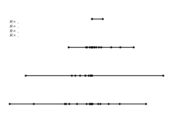
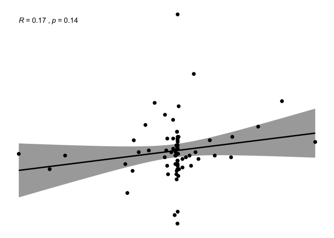
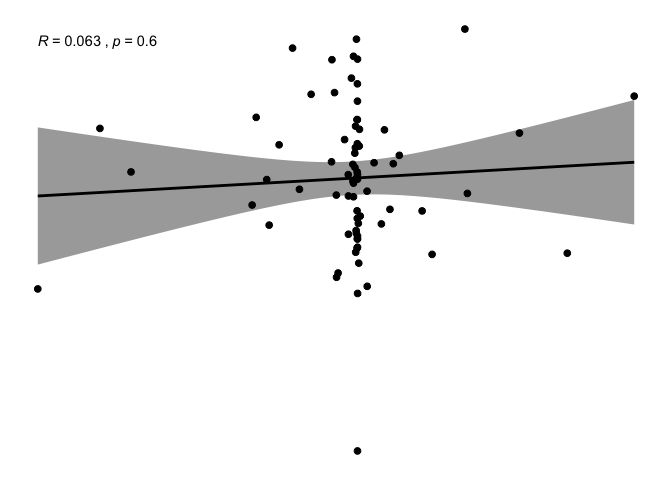
We can eye-ball the relationship between our dependent variable and the independent ones:
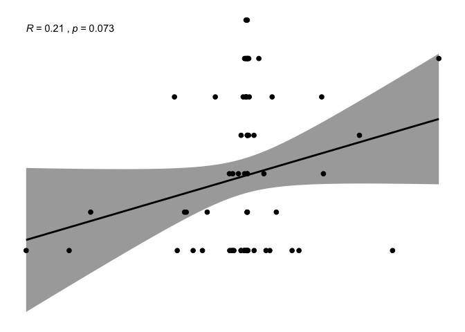
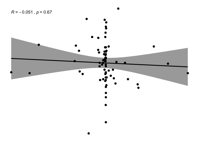
ggscatter(newREDD, x = "def", y = "rpp",
          add = "reg.line", conf.int = TRUE,
          cor.coef = TRUE, cor.method = "pearson",
          xlab = "deforestation progress between 2010 and 2015", ylab = "anteriority of RPP")
ggscatter(newREDD, x = "def", y = "fund",
          add = "reg.line", conf.int = TRUE,
          cor.coef = TRUE, cor.method = "pearson",
          xlab = "deforestation progress between 2010 and 2015", ylab = "Funds joined by REDD+ countries")
ggscatter(newREDD, x = "def", y = "fpic",
          add = "reg.line", conf.int = TRUE,
          cor.coef = TRUE, cor.method = "pearson",
          xlab = "deforestation progress between 2010 and 2015", ylab = "Presence of FPIC in REDD+ projects")
ggscatter(newREDD, x = "def", y = "part",
          add = "reg.line", conf.int = TRUE,
          cor.coef = TRUE, cor.method = "pearson",
          xlab = "deforestation progress between 2010 and 2015", ylab = "Use of participatory approaches")
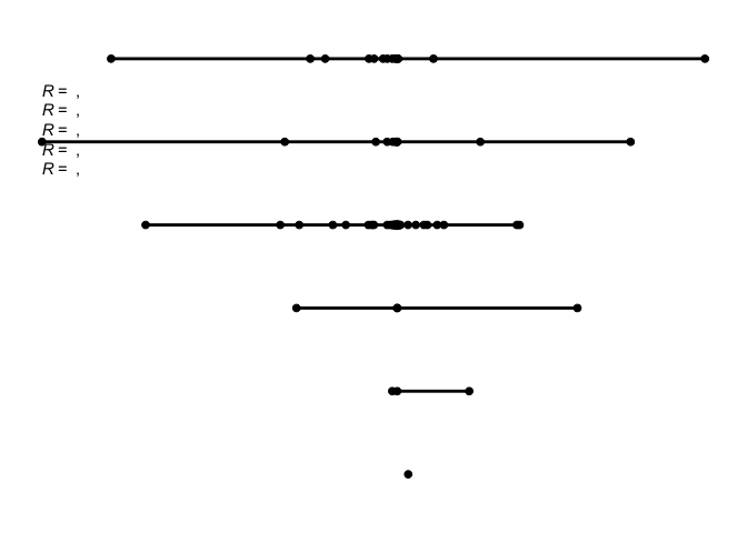
ggscatter(newREDD, x = "def", y = "continent",
          add = "reg.line", conf.int = TRUE,
          cor.coef = TRUE, cor.method = "pearson",
          xlab = "deforestation progress between 2010 and 2015", ylab = "Continent")
ggscatter(newREDD, x = "def", y = "projects",
          add = "reg.line", conf.int = TRUE,
          cor.coef = TRUE, cor.method = "pearson",
          xlab = "deforestation progress between 2010 and 2015", ylab = "Number of REDD+ projects")
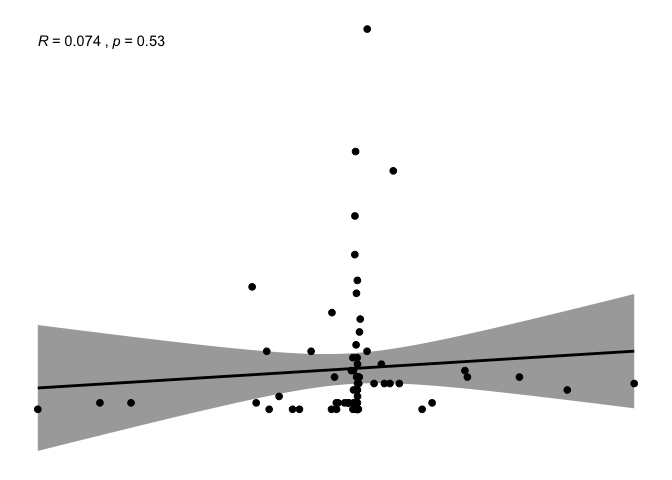
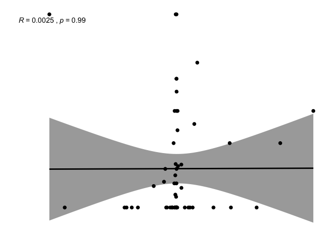
ggscatter(newREDD, x = "def", y = "IDH",
          add = "reg.line", conf.int = TRUE,
          cor.coef = TRUE, cor.method = "pearson",
          xlab = "deforestation progress between 2010 and 2015", ylab = "IDH progress")
ggscatter(newREDD, x = "def", y = "GDPhab",
          add = "reg.line", conf.int = TRUE,
          cor.coef = TRUE, cor.method = "pearson",
          xlab = "deforestation progress between 2010 and 2015", ylab = "GDP per capita progress")
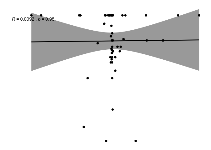
ggscatter(newREDD, x = "def", y = "Gov",
          add = "reg.line", conf.int = TRUE,
          cor.coef = TRUE, cor.method = "pearson",
          xlab = "deforestation progress between 2010 and 2015", ylab = "Government effectiveness progress")
ggscatter(newREDD, x = "def", y = "Corrupt",
          add = "reg.line", conf.int = TRUE,
          cor.coef = TRUE, cor.method = "pearson",
          xlab = "deforestation progress between 2010 and 2015", ylab = "Corruption control progress")
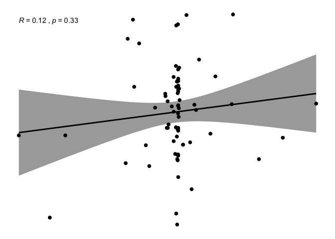
It is really difficult to eye-ball any pattern on these variables and they seem very scattered, with powerful outliers. Some transformation and imputation is needed.
Treating lagged effects
The REDD+ related variables (“fund”, “fpic”, and “part”, and “projects”) may have a lagged effect, as between the start date of the signature of an agreement or the launch of a project, an FPIC protocole or the related participatory approaches, there may be some delay before they start having an effect on deforestation rates.
newREDD$fund <- lag(newREDD$fund, 1)
newREDD$projects <- lag(newREDD$projects, 1)
newREDD$fpic <- lag(newREDD$fpic, 1)
newREDD$part <- lag(newREDD$part, 1)
Diagnosing and treating missing data
sapply(newREDD, function(x) sum(is.na(x)))
country_name continent fund rpp projects IDH 0 0 1 0 1 1 GDPhab Corrupt rpp_date id_country fpic part 0 1 0 0 17 17 def Gov 0 0 There are 17 missing data for fpic and 17 for part, 1 for IDH, 1 for projects, 1 for corrupt, 1 for fund, over a total of 74 observations. They may matter for fpic and part. Because I would like to avoid “crude and cruel” ways to treat missing data by imputing values (mean, median or mode), I will treat them using rpart for fpic and part. As per the 1 missing value for IDH, projects and corrupt, they are linked to the same observation on South Sudan. This observation being problematic (5 missing values), and South Sudan being a particular country where it is hard to have reliable data at the moment due to the on-going geopolitical situation, I will exclude this country from the dataset to build my models. After deleting this one observation over 74, the dataset will still have sufficent data points, so the model won’t lose power, and it will avoid introducing bias.
newREDD <- newREDD[-c(60),]
miceMod <- mice(newREDD[, !names(newREDD) %in% "fpic"], method="rf")
iter imp variable 1 1 fund projects IDH Corrupt part 1 2 fund projects IDH Corrupt part 1 3 fund projects IDH Corrupt part 1 4 fund projects IDH Corrupt part 1 5 fund projects IDH Corrupt part 2 1 fund projects IDH Corrupt part 2 2 fund projects IDH Corrupt part 2 3 fund projects IDH Corrupt part 2 4 fund projects IDH Corrupt part 2 5 fund projects IDH Corrupt part 3 1 fund projects IDH Corrupt part 3 2 fund projects IDH Corrupt part 3 3 fund projects IDH Corrupt part 3 4 fund projects IDH Corrupt part 3 5 fund projects IDH Corrupt part 4 1 fund projects IDH Corrupt part 4 2 fund projects IDH Corrupt part 4 3 fund projects IDH Corrupt part 4 4 fund projects IDH Corrupt part 4 5 fund projects IDH Corrupt part 5 1 fund projects IDH Corrupt part 5 2 fund projects IDH Corrupt part 5 3 fund projects IDH Corrupt part 5 4 fund projects IDH Corrupt part 5 5 fund projects IDH Corrupt part
miceOutput <- complete(miceMod)
anyNA(miceOutput)
[1] FALSE
miceMod <- mice(newREDD[, !names(newREDD) %in% "part"], method="rf")
iter imp variable 1 1 fund projects IDH Corrupt fpic 1 2 fund projects IDH Corrupt fpic 1 3 fund projects IDH Corrupt fpic 1 4 fund projects IDH Corrupt fpic 1 5 fund projects IDH Corrupt fpic 2 1 fund projects IDH Corrupt fpic 2 2 fund projects IDH Corrupt fpic 2 3 fund projects IDH Corrupt fpic 2 4 fund projects IDH Corrupt fpic 2 5 fund projects IDH Corrupt fpic 3 1 fund projects IDH Corrupt fpic 3 2 fund projects IDH Corrupt fpic 3 3 fund projects IDH Corrupt fpic 3 4 fund projects IDH Corrupt fpic 3 5 fund projects IDH Corrupt fpic 4 1 fund projects IDH Corrupt fpic 4 2 fund projects IDH Corrupt fpic 4 3 fund projects IDH Corrupt fpic 4 4 fund projects IDH Corrupt fpic 4 5 fund projects IDH Corrupt fpic 5 1 fund projects IDH Corrupt fpic 5 2 fund projects IDH Corrupt fpic 5 3 fund projects IDH Corrupt fpic 5 4 fund projects IDH Corrupt fpic 5 5 fund projects IDH Corrupt fpic
miceOutput <- complete(miceMod)
anyNA(miceOutput)
[1] FALSE
Lets compute the accuracy of fpic and part now.
actuals <- REDD$fpic[is.na(newREDD$fpic)]
predicteds <- miceOutput[is.na(newREDD$fpic), "fpic"]
regr.eval(actuals, predicteds)
mae mse rmse mape NA NA NA NA
actuals <- REDD$part[is.na(newREDD$part)]
predicteds <- miceOutput[is.na(newREDD$part), "part"]
regr.eval(actuals, predicteds)
mae mse rmse mape 0 0 0 0
I expected the mean absolute percentage error (mape) to improve. There seems to be a problem, and I can’t run alternative code such as rpart, so I will assume this is correct!
3. Methods
To answer the research question I propose linear regression models, one based on REDD+ projects-related variables, the second one on governance and socio-economic variables, and the third one combining all variables. I would like to know if REDD+ based variables only can be good predictors, or overall governance indicators, or alternatively if a mix of both could predict better the deforestation progress.
lm1 <-lm(def~fund+rpp+projects+fpic+part, data=newREDD)
lm2 <-lm(def~IDH+GDPhab+Gov+Corrupt, data=newREDD)
lm3 <-lm(def~fund+rpp+projects+fpic+part+IDH+GDPhab+Gov+Corrupt, data=newREDD)
summary(lm1)
Call: lm(formula = def ~ fund + rpp + projects + fpic + part, data = newREDD)
Residuals: Min 1Q Median 3Q Max -2.8112 -0.3249 -0.1746 0.5412 3.0490
Coefficients: Estimate Std. Error t value Pr(>|t|) (Intercept) 0.305940 1.496357 0.204 0.839 fundCongo Basin Forest Fund;FCPF;UNREDD 0.857890 1.480061 0.580 0.565 fundFCPF -1.220345 1.499869 -0.814 0.420 fundFCPF;UNREDD -0.039164 1.378093 -0.028 0.977 fundNo -0.554748 1.429671 -0.388 0.700 fundUNREDD 0.354498 1.439186 0.246 0.807 rpp 0.077090 0.091319 0.844 0.403 projects -0.001191 0.016943 -0.070 0.944 fpic 0.144073 0.544475 0.265 0.792 part -0.481237 0.617481 -0.779 0.440
Residual standard error: 1.031 on 46 degrees of freedom (17 observations deleted due to missingness) Multiple R-squared: 0.2001, Adjusted R-squared: 0.04363 F-statistic: 1.279 on 9 and 46 DF, p-value: 0.274
summary(lm2)
Call: lm(formula = def ~ IDH + GDPhab + Gov + Corrupt, data = newREDD)
Residuals: Min 1Q Median 3Q Max -4.0645 -0.2055 0.0576 0.4201 3.5745
Coefficients: Estimate Std. Error t value Pr(>|t|) (Intercept) -1.3409 1.4682 -0.913 0.364 IDH 12.7506 7.8461 1.625 0.109 GDPhab 0.9567 1.3445 0.712 0.479 Gov -0.5314 0.5736 -0.926 0.358 Corrupt 0.1659 0.1659 1.000 0.321
Residual standard error: 1.09 on 67 degrees of freedom (1 observation deleted due to missingness) Multiple R-squared: 0.06086, Adjusted R-squared: 0.004788 F-statistic: 1.085 on 4 and 67 DF, p-value: 0.3709
summary(lm3)
Call: lm(formula = def ~ fund + rpp + projects + fpic + part + IDH + GDPhab + Gov + Corrupt, data = newREDD)
Residuals: Min 1Q Median 3Q Max -2.84218 -0.48925 -0.00564 0.46381 3.00524
Coefficients: Estimate Std. Error t value Pr(>|t|)
(Intercept) -0.01021 2.16557 -0.005 0.9963
fundCongo Basin Forest Fund;FCPF;UNREDD 1.76360 1.43790 1.227 0.2268
fundFCPF -0.61094 1.43511 -0.426 0.6725
fundFCPF;UNREDD 0.31410 1.30547 0.241 0.8110
fundNo 0.51398 1.39539 0.368 0.7145
fundUNREDD 0.95775 1.37667 0.696 0.4904
rpp 0.16881 0.09156 1.844 0.0723 . projects 0.01350 0.01671 0.808
0.4236
fpic 0.61655 0.53542 1.152 0.2560
part -0.39251 0.58881 -0.667 0.5087
IDH 14.17490 7.64361 1.854 0.0707 . GDPhab -0.86167 1.61529 -0.533
0.5965
Gov -1.85656 0.76544 -2.425 0.0197 * Corrupt 0.16738 0.17655 0.948
0.3485
— Signif. codes: 0 ‘’ 0.001 ’’ 0.01 ’’ 0.05 ‘.’ 0.1 ’ ’ 1
Residual standard error: 0.9644 on 42 degrees of freedom (17 observations deleted due to missingness) Multiple R-squared: 0.3614, Adjusted R-squared: 0.1637 F-statistic: 1.828 on 13 and 42 DF, p-value: 0.07013
tab_model(lm1)
| deforestation rate evolution 2010-2015 | |||
|---|---|---|---|
| Predictors | Estimates | CI | p |
| (Intercept) | 0.31 | -2.71 – 3.32 | 0.839 |
| Agreement with international REDD+ funds: Congo Basin Forest Fund;FCPF;UNREDD | 0.86 | -2.12 – 3.84 | 0.565 |
| Agreement with international REDD+ funds: FCPF | -1.22 | -4.24 – 1.80 | 0.420 |
| Agreement with international REDD+ funds: FCPF;UNREDD | -0.04 | -2.81 – 2.73 | 0.977 |
| Agreement with international REDD+ funds: No | -0.55 | -3.43 – 2.32 | 0.700 |
| Agreement with international REDD+ funds: UNREDD | 0.35 | -2.54 – 3.25 | 0.807 |
| Anteriority of RPP | 0.08 | -0.11 – 0.26 | 0.403 |
| Number of REDD+ projects | -0.00 | -0.04 – 0.03 | 0.944 |
| Free Prior Informed Consent index | 0.14 | -0.95 – 1.24 | 0.792 |
| Participatory approaches index | -0.48 | -1.72 – 0.76 | 0.440 |
| Observations | 56 | ||
| R2 / R2 adjusted | 0.200 / 0.044 | ||
| deforestation rate evolution 2010-2015 | |||
|---|---|---|---|
| Predictors | Estimates | CI | p |
| (Intercept) | -1.34 | -4.27 – 1.59 | 0.364 |
| IDH progress | 12.75 | -2.91 – 28.41 | 0.109 |
| GDP per capita progress | 0.96 | -1.73 – 3.64 | 0.479 |
| Government effectiveness progress | -0.53 | -1.68 – 0.61 | 0.358 |
| Corruption control progress | 0.17 | -0.17 – 0.50 | 0.321 |
| Observations | 72 | ||
| R2 / R2 adjusted | 0.061 / 0.005 | ||
| deforestation rate evolution 2010-2015 | |||
|---|---|---|---|
| Predictors | Estimates | CI | p |
| (Intercept) | -0.01 | -4.38 – 4.36 | 0.996 |
| Agreement with international REDD+ funds: Congo Basin Forest Fund;FCPF;UNREDD | 1.76 | -1.14 – 4.67 | 0.227 |
| Agreement with international REDD+ funds: FCPF | -0.61 | -3.51 – 2.29 | 0.672 |
| Agreement with international REDD+ funds: FCPF;UNREDD | 0.31 | -2.32 – 2.95 | 0.811 |
| Agreement with international REDD+ funds: No | 0.51 | -2.30 – 3.33 | 0.714 |
| Agreement with international REDD+ funds: UNREDD | 0.96 | -1.82 – 3.74 | 0.490 |
| Anteriority of RPP | 0.17 | -0.02 – 0.35 | 0.072 |
| Number of REDD+ projects | 0.01 | -0.02 – 0.05 | 0.424 |
| Free Prior Informed Consent index | 0.62 | -0.46 – 1.70 | 0.256 |
| Participatory approaches index | -0.39 | -1.58 – 0.80 | 0.509 |
| IDH progress | 14.17 | -1.25 – 29.60 | 0.071 |
| GDP per capita progress | -0.86 | -4.12 – 2.40 | 0.597 |
| Government effectiveness progress | -1.86 | -3.40 – -0.31 | 0.020 |
| Corruption control progress | 0.17 | -0.19 – 0.52 | 0.349 |
| Observations | 56 | ||
| R2 / R2 adjusted | 0.361 / 0.164 | ||
According to the theorem, there are a series of assumptions that I need to check, potentially having to treat arising issues within the dataset:
Outliers
car::outlierTest(lm1)
rstudent unadjusted p-value Bonferroni p 35 4.033947 0.00020985 0.011542
car::outlierTest(lm2)

rstudent unadjusted p-value Bonferroni p
67 -4.301293 5.7334e-05 0.0041281 35 3.660775 5.0150e-04 0.0361080
car::outlierTest(lm3)

rstudent unadjusted p-value Bonferroni p
49 4.118279 0.00018025 0.0099137 50 -4.103705 0.00018847 0.0103660
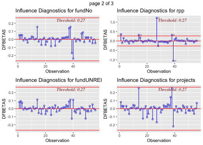
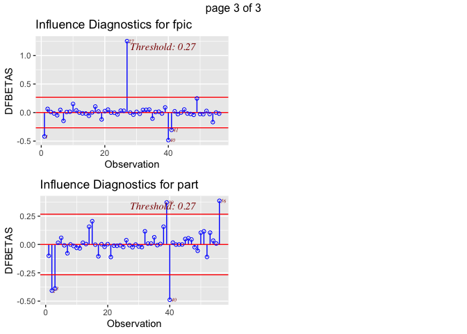
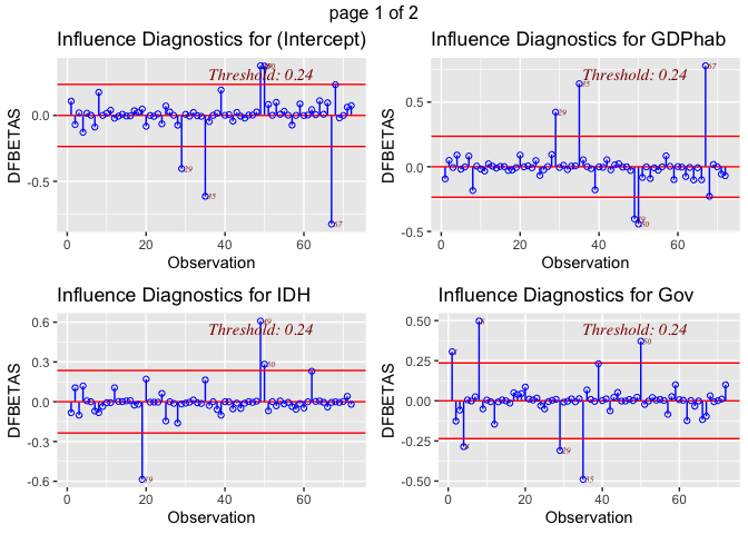
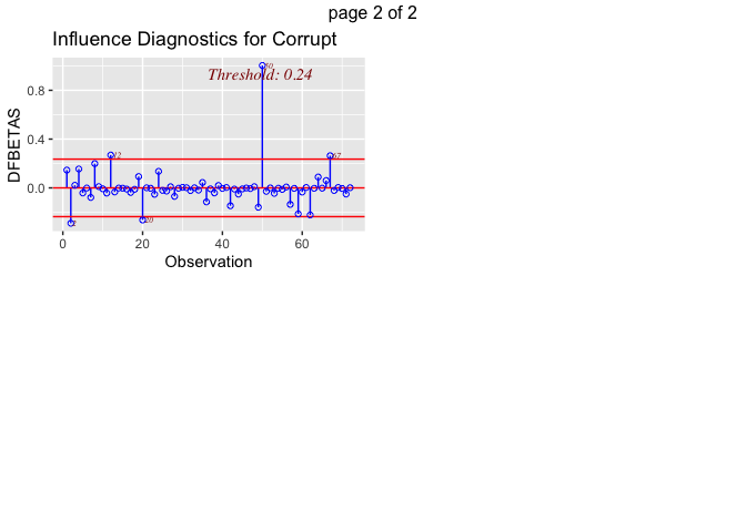
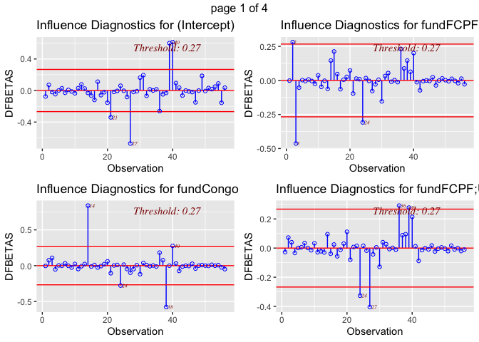
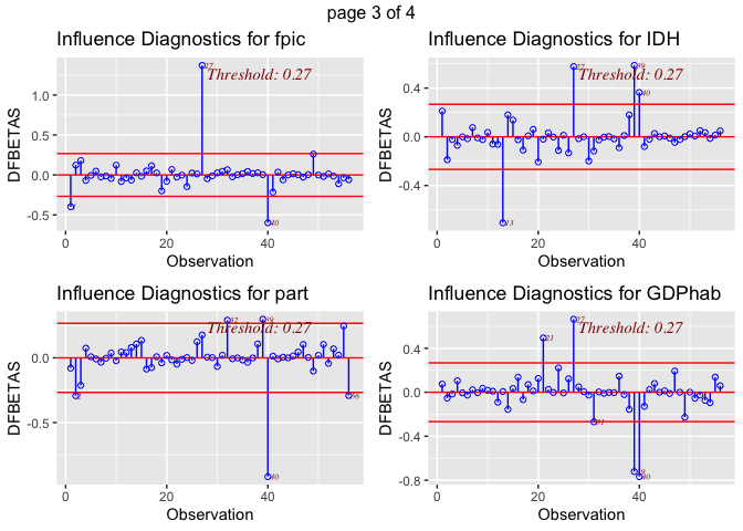
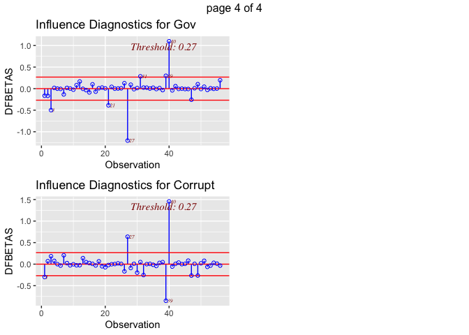
dfbetaPlots(lm1)
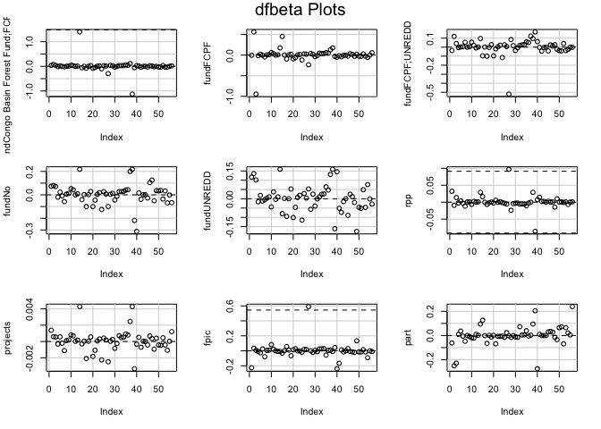
dfbetaPlots(lm2)
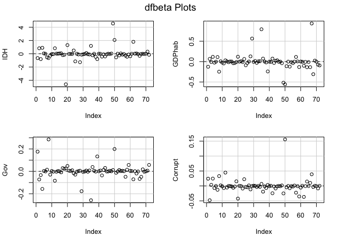
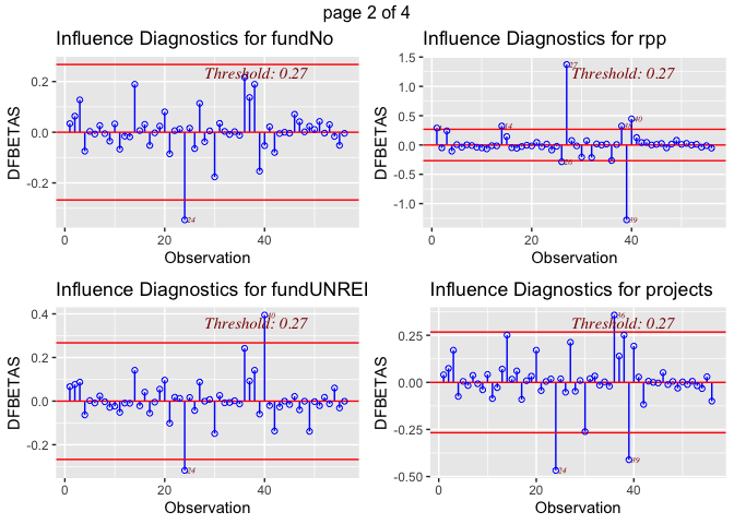
dfbetaPlots(lm3)
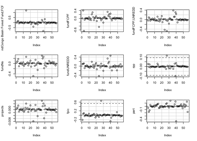
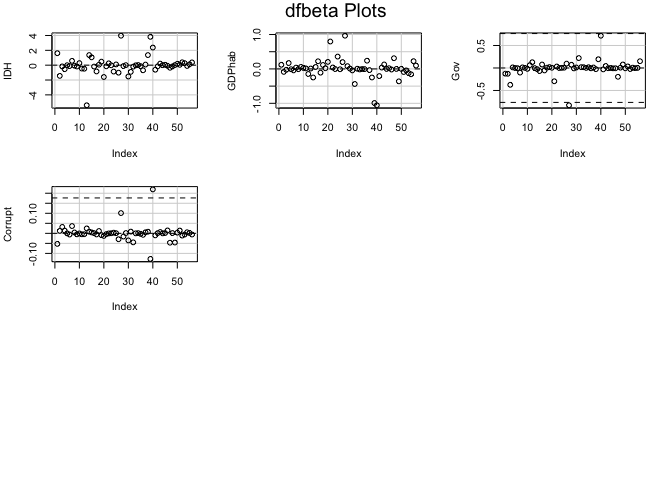 The dfbetas plots illustrate that there are outliers within the variable
def (deforestation progress between 2010 and 2015). The most concerning
outliers are Burundi, with a negative index on its deforestation rate
progress, and Philippines, which has a high value. Both could have a
disproportionate impact on results. Although, it is not clear how much
each of these outliers influence the regression model. Also, looking at
the dfbeta plots it appears that outliers are also present in the some
of the other variables used in the model. This is why we will use a
Cook’s D to find out if this outlier really matters for the regression
models.
The dfbetas plots illustrate that there are outliers within the variable
def (deforestation progress between 2010 and 2015). The most concerning
outliers are Burundi, with a negative index on its deforestation rate
progress, and Philippines, which has a high value. Both could have a
disproportionate impact on results. Although, it is not clear how much
each of these outliers influence the regression model. Also, looking at
the dfbeta plots it appears that outliers are also present in the some
of the other variables used in the model. This is why we will use a
Cook’s D to find out if this outlier really matters for the regression
models.
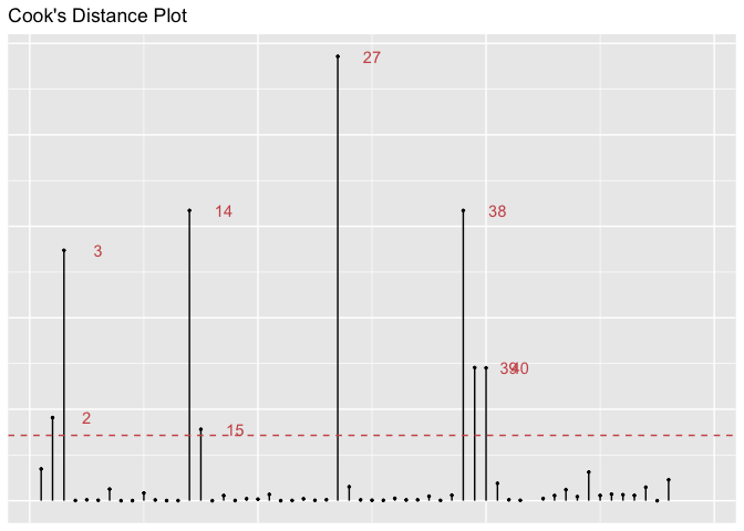
gg_cooksd(lm1)
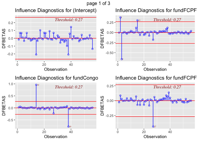
ols_plot_dfbetas(lm1)
gg_cooksd(lm2)
ols_plot_dfbetas(lm2)
gg_cooksd(lm3)
ols_plot_dfbetas(lm3)
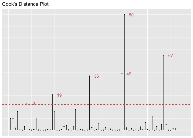
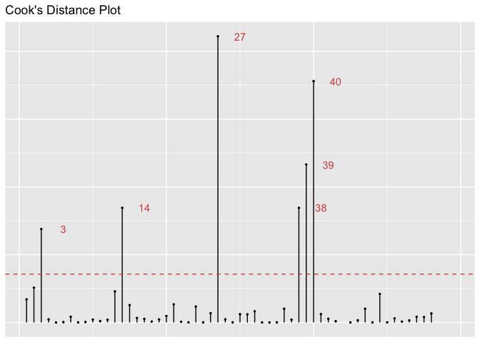
 The Cook’s D plot illustrates that some variables do influence our
regression models’ results. This appears to be the case for variables
number 2 (Bengladesh), 3 (Belize), 8 (Burkina Faso), 14 (Chad), 19
(DRC), 27(Guatemala), 35 (Liberia), 38 (Malaysia), 39 (Mali),
40(Mexico), 49 (Panama), 50 (PNG), 67 (Uganda)). The Cook’s D plot is
telling us is how much deleting each observation would influence the
predicted outcome of the model. However, so many outliers (more than 10%
of the dataset) could also mean that we are with a dataset with a lot of
variation, and not in front of real outliers. This is confirmed by the
diversity of observations: we are dealing with different countries, on
different continents. In addition, there does not seem to be any pattern
in those observations (for instance, countries from one continent only).
We can then conclude that these values are no longer outliers. According
to the dfbetatest, Philippines and Burundi could deserve some more focus
in further studies - their values may be related to the particular
situation of these countries, to be investigated. In order to make sure
that these outliers do not influence the model too much, we can compare
the results with and without them.
The Cook’s D plot illustrates that some variables do influence our
regression models’ results. This appears to be the case for variables
number 2 (Bengladesh), 3 (Belize), 8 (Burkina Faso), 14 (Chad), 19
(DRC), 27(Guatemala), 35 (Liberia), 38 (Malaysia), 39 (Mali),
40(Mexico), 49 (Panama), 50 (PNG), 67 (Uganda)). The Cook’s D plot is
telling us is how much deleting each observation would influence the
predicted outcome of the model. However, so many outliers (more than 10%
of the dataset) could also mean that we are with a dataset with a lot of
variation, and not in front of real outliers. This is confirmed by the
diversity of observations: we are dealing with different countries, on
different continents. In addition, there does not seem to be any pattern
in those observations (for instance, countries from one continent only).
We can then conclude that these values are no longer outliers. According
to the dfbetatest, Philippines and Burundi could deserve some more focus
in further studies - their values may be related to the particular
situation of these countries, to be investigated. In order to make sure
that these outliers do not influence the model too much, we can compare
the results with and without them.
newREDDO <- newREDD[-c(10,54),]
lm1O <- lm(def~fund+rpp+projects+fpic+part, data=newREDDO)
lm2O <-lm(def~IDH+GDPhab+Gov+Corrupt, data=newREDDO)
lm3O <-lm(def~fund+rpp+projects+fpic+part+IDH+GDPhab+Gov+Corrupt, data=newREDDO)
tab_model(lm1, lm1O, dv.labels = c("Fertility With Outliers","Fertility Without"))
| Fertility With Outliers | Fertility Without | |||||
|---|---|---|---|---|---|---|
| Predictors | Estimates | CI | p | Estimates | CI | p |
| (Intercept) | 0.31 | -2.71 – 3.32 | 0.839 | 1.20 | -0.66 – 3.06 | 0.201 |
| Agreement with international REDD+ funds: Congo Basin Forest Fund;FCPF;UNREDD | 0.86 | -2.12 – 3.84 | 0.565 | |||
| Agreement with international REDD+ funds: FCPF | -1.22 | -4.24 – 1.80 | 0.420 | -2.08 | -4.04 – -0.13 | 0.037 |
| Agreement with international REDD+ funds: FCPF;UNREDD | -0.04 | -2.81 – 2.73 | 0.977 | -0.88 | -2.46 – 0.70 | 0.267 |
| Agreement with international REDD+ funds: No | -0.55 | -3.43 – 2.32 | 0.700 | -1.42 | -3.11 – 0.27 | 0.097 |
| Agreement with international REDD+ funds: UNREDD | 0.35 | -2.54 – 3.25 | 0.807 | -0.51 | -2.21 – 1.20 | 0.554 |
| Anteriority of RPP | 0.08 | -0.11 – 0.26 | 0.403 | 0.07 | -0.11 – 0.26 | 0.436 |
| Number of REDD+ projects | -0.00 | -0.04 – 0.03 | 0.944 | -0.00 | -0.04 – 0.03 | 0.919 |
| Free Prior Informed Consent index | 0.14 | -0.95 – 1.24 | 0.792 | 0.17 | -0.96 – 1.30 | 0.762 |
| Participatory approaches index | -0.48 | -1.72 – 0.76 | 0.440 | -0.52 | -1.81 – 0.77 | 0.423 |
| Observations | 56 | 54 | ||||
| R2 / R2 adjusted | 0.200 / 0.044 | 0.201 / 0.059 | ||||
| Fertility With Outliers | Fertility Without | |||||
|---|---|---|---|---|---|---|
| Predictors | Estimates | CI | p | Estimates | CI | p |
| (Intercept) | -1.34 | -4.27 – 1.59 | 0.364 | -1.38 | -4.39 – 1.64 | 0.365 |
| IDH progress | 12.75 | -2.91 – 28.41 | 0.109 | 12.76 | -3.21 – 28.74 | 0.115 |
| GDP per capita progress | 0.96 | -1.73 – 3.64 | 0.479 | 0.99 | -1.77 – 3.76 | 0.476 |
| Government effectiveness progress | -0.53 | -1.68 – 0.61 | 0.358 | -0.54 | -1.70 – 0.63 | 0.361 |
| Corruption control progress | 0.17 | -0.17 – 0.50 | 0.321 | 0.17 | -0.17 – 0.50 | 0.324 |
| Observations | 72 | 70 | ||||
| R2 / R2 adjusted | 0.061 / 0.005 | 0.061 / 0.003 | ||||
| Fertility With Outliers | Fertility Without | |||||
|---|---|---|---|---|---|---|
| Predictors | Estimates | CI | p | Estimates | CI | p |
| (Intercept) | -0.01 | -4.38 – 4.36 | 0.996 | 1.75 | -2.51 – 6.01 | 0.412 |
| Agreement with international REDD+ funds: Congo Basin Forest Fund;FCPF;UNREDD | 1.76 | -1.14 – 4.67 | 0.227 | |||
| Agreement with international REDD+ funds: FCPF | -0.61 | -3.51 – 2.29 | 0.672 | -2.37 | -4.28 – -0.47 | 0.016 |
| Agreement with international REDD+ funds: FCPF;UNREDD | 0.31 | -2.32 – 2.95 | 0.811 | -1.45 | -3.00 – 0.11 | 0.068 |
| Agreement with international REDD+ funds: No | 0.51 | -2.30 – 3.33 | 0.714 | -1.25 | -2.86 – 0.36 | 0.124 |
| Agreement with international REDD+ funds: UNREDD | 0.96 | -1.82 – 3.74 | 0.490 | -0.81 | -2.44 – 0.83 | 0.327 |
| Anteriority of RPP | 0.17 | -0.02 – 0.35 | 0.072 | 0.17 | -0.02 – 0.36 | 0.081 |
| Number of REDD+ projects | 0.01 | -0.02 – 0.05 | 0.424 | 0.01 | -0.02 – 0.05 | 0.437 |
| Free Prior Informed Consent index | 0.62 | -0.46 – 1.70 | 0.256 | 0.62 | -0.49 – 1.73 | 0.265 |
| Participatory approaches index | -0.39 | -1.58 – 0.80 | 0.509 | -0.40 | -1.63 – 0.83 | 0.518 |
| IDH progress | 14.17 | -1.25 – 29.60 | 0.071 | 14.18 | -1.45 – 29.80 | 0.074 |
| GDP per capita progress | -0.86 | -4.12 – 2.40 | 0.597 | -0.85 | -4.18 – 2.48 | 0.608 |
| Government effectiveness progress | -1.86 | -3.40 – -0.31 | 0.020 | -1.86 | -3.42 – -0.29 | 0.021 |
| Corruption control progress | 0.17 | -0.19 – 0.52 | 0.349 | 0.17 | -0.19 – 0.53 | 0.354 |
| Observations | 56 | 54 | ||||
| R2 / R2 adjusted | 0.361 / 0.164 | 0.361 / 0.174 | ||||
normality
Let’s check if the residuals are normally distributed, first by eye-balling the distribution, and then by performing a formal test
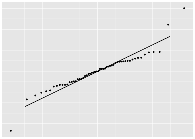
df_resid <- data.frame(resid = lm1$residuals)
p <- ggplot(df_resid, aes(sample = resid))
p + stat_qq() + stat_qq_line()
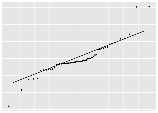
ols_test_normality(lm1)
| Test Statistic pvalue |
|---|
| Shapiro-Wilk 0.8965 2e-04 Kolmogorov-Smirnov 0.1607 0.0990 Cramer-von Mises 6.7727 0.0000 Anderson-Darling 2.0166 0.0000 |
It seems a little bit off at both ends.
df_resid <- data.frame(resid = lm2$residuals)
p <- ggplot(df_resid, aes(sample = resid))
p + stat_qq() + stat_qq_line()
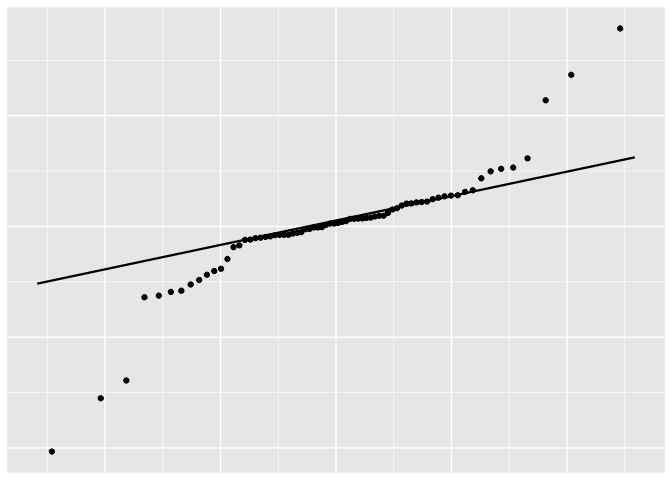
ols_test_normality(lm2)
| Test Statistic pvalue |
|---|
| Shapiro-Wilk 0.8512 0.0000 Kolmogorov-Smirnov 0.2007 0.0051 Cramer-von Mises 6.922 0.0000 Anderson-Darling 3.7186 0.0000 |
Again, it is a little bit off at both ends.
df_resid <- data.frame(resid = lm3$residuals)
p <- ggplot(df_resid, aes(sample = resid))
p + stat_qq() + stat_qq_line()
ols_test_normality(lm3)
| Test Statistic pvalue |
|---|
| Shapiro-Wilk 0.919 0.0011 Kolmogorov-Smirnov 0.1151 0.4166 Cramer-von Mises 5.0521 0.0000 Anderson-Darling 1.0218 0.0100 |
This is quite normally distributed, but a little off at one end.
Only by looking at the residuals plot it is hard to say whether the residuals are indeed normally distributed - the ends look a bit off. However, after performing the formal tests too, we fail to reject the null hypothesis that residuals are normally distributed. This means we can proceed with the assumption that residuals are normally distributed.
non-linearity
plotpreds <- function(lm1, data = Data){
p1 <- ggplot(lm1, aes(.fitted, .resid)) +
  geom_point() +
  stat_smooth(method="loess") +
  geom_hline(yintercept=0, col="red") +
  xlab("Predicted") + ylab("Residuals") +
  ggtitle("Residuals vs. Predicted Values")
df_plt <- data.frame("fitted" = fitted(lm5),
                  "observed" = newREDD$def)
p2 <- ggplot(df_plt, aes(x=fitted, y=observed)) +
  geom_point() + stat_smooth(method="loess") +
  geom_abline(intercept = 1, col="red") +
  xlab("Predicted") + ylab("Observed") +
  ggtitle("Observed vs. Predicted Values")
grid.arrange(p1, p2, ncol=2)
}

plotpreds <- function(lm2, data = Data){
p1 <- ggplot(lm1, aes(.fitted, .resid)) +
  geom_point() +
  stat_smooth(method="loess") +
  geom_hline(yintercept=0, col="red") +
  xlab("Predicted") + ylab("Residuals") +
  ggtitle("Residuals vs. Predicted Values")
df_plt <- data.frame("fitted" = fitted(lm5),
                  "observed" = newREDD$def)
p2 <- ggplot(df_plt, aes(x=fitted, y=observed)) +
  geom_point() + stat_smooth(method="loess") +
  geom_abline(intercept = 1, col="red") +
  xlab("Predicted") + ylab("Observed") +
  ggtitle("Observed vs. Predicted Values")
grid.arrange(p1, p2, ncol=2)
}

plotpreds <- function(lm3, data = Data){
p1 <- ggplot(lm1, aes(.fitted, .resid)) +
  geom_point() +
  stat_smooth(method="loess") +
  geom_hline(yintercept=0, col="red") +
  xlab("Predicted") + ylab("Residuals") +
  ggtitle("Residuals vs. Predicted Values")
df_plt <- data.frame("fitted" = fitted(lm5),
                  "observed" = newREDD$def)
p2 <- ggplot(df_plt, aes(x=fitted, y=observed)) +
  geom_point() + stat_smooth(method="loess") +
  geom_abline(intercept = 1, col="red") +
  xlab("Predicted") + ylab("Observed") +
  ggtitle("Observed vs. Predicted Values")
grid.arrange(p1, p2, ncol=2)
}
I expect the three models to be linear. However, once again I am unable to run these codes and interpret the results so I will assume linearity.
checking bias
Deforestation rate is not a cause of the other variables, so we assume that there is no simultaneity bias. There could be a measurement errorr because of the changes we made (suppressing South Sudan and treating the outliers). However, the countries that were causing troubles in the dataset were from diverse regions and continent, hence this does not constitute a statistically significant bias. We could check auto-correlation to make sure this is not an issue.
lmtest::dwtest(lm2)

Durbin-Watson test
data: lm2 DW = 2.1247, p-value = 0.6829 alternative hypothesis: true autocorrelation is greater than 0
ggAcf(lm1$residuals)
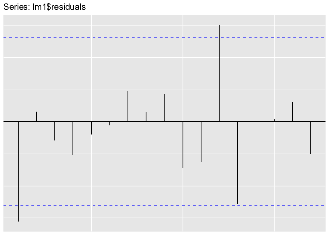
lmtest::dwtest(lm1)

Durbin-Watson test
data: lm1 DW = 2.5856, p-value = 0.9729 alternative hypothesis: true autocorrelation is greater than 0
lawstat::runs.test(lm1$residuals)

Runs Test - Two sided
data: lm1$residuals Standardized Runs Statistic = -0.53945, p-value = 0.5896
ggAcf(lm2$residuals)
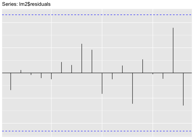
lawstat::runs.test(lm2$residuals)

Runs Test - Two sided
data: lm2$residuals Standardized Runs Statistic = -0.47476, p-value = 0.635
ggAcf(lm3$residuals)
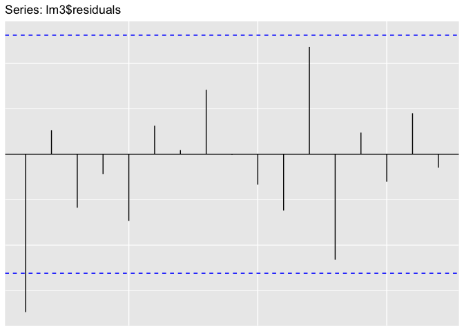
lmtest::dwtest(lm3)

Durbin-Watson test
data: lm3 DW = 2.669, p-value = 0.9872 alternative hypothesis: true autocorrelation is greater than 0
lawstat::runs.test(lm3$residuals)

Runs Test - Two sided
data: lm3$residuals Standardized Runs Statistic = 1.3486, p-value = 0.1775 There are no apparent bias.
heteroskedasticity
bptest(lm1, data=demo, studentize = TRUE)

studentized Breusch-Pagan test
data: lm1 BP = 8.6494, df = 9, p-value = 0.4702
gvlma::gvlma(lm1)
Call: lm(formula = def ~ fund + rpp + projects + fpic + part, data = newREDD)
Coefficients: (Intercept)
0.305940
fundCongo Basin Forest Fund;FCPF;UNREDD
0.857890
fundFCPF
-1.220345
fundFCPF;UNREDD
-0.039164
fundNo
-0.554748
fundUNREDD
0.354498
rpp
0.077090
projects
-0.001191
fpic
0.144073
part
-0.481237
ASSESSMENT OF THE LINEAR MODEL ASSUMPTIONS USING THE GLOBAL TEST ON 4 DEGREES-OF-FREEDOM: Level of Significance = 0.05
Call: gvlma::gvlma(x = lm1)
Value p-value Decision
Global Stat 28.9221 8.108e-06 Assumptions NOT satisfied! Skewness 4.3119 3.785e-02 Assumptions NOT satisfied! Kurtosis 23.9877 9.695e-07 Assumptions NOT satisfied! Link Function 0.3716 5.422e-01 Assumptions acceptable. Heteroscedasticity 0.2509 6.164e-01 Assumptions acceptable.
bptest(lm2, data=demo, studentize = TRUE)

studentized Breusch-Pagan test
data: lm2 BP = 2.7453, df = 4, p-value = 0.6013
gvlma::gvlma(lm2)
Call: lm(formula = def ~ IDH + GDPhab + Gov + Corrupt, data = newREDD)
Coefficients: (Intercept) IDH GDPhab Gov Corrupt
-1.3409 12.7506 0.9567 -0.5314 0.1659
ASSESSMENT OF THE LINEAR MODEL ASSUMPTIONS USING THE GLOBAL TEST ON 4 DEGREES-OF-FREEDOM: Level of Significance = 0.05
Call: gvlma::gvlma(x = lm2)
Value p-value Decision
Global Stat 75.34200 1.665e-15 Assumptions NOT satisfied! Skewness 3.33382 6.787e-02 Assumptions acceptable. Kurtosis 70.62266 0.000e+00 Assumptions NOT satisfied! Link Function 0.06251 8.026e-01 Assumptions acceptable. Heteroscedasticity 1.32302 2.501e-01 Assumptions acceptable.
bptest(lm3, data=demo, studentize = TRUE)

studentized Breusch-Pagan test
data: lm3 BP = 11.781, df = 13, p-value = 0.5457
gvlma::gvlma(lm3)
Call: lm(formula = def ~ fund + rpp + projects + fpic + part + IDH + GDPhab + Gov + Corrupt, data = newREDD)
Coefficients: (Intercept)
-0.01021
fundCongo Basin Forest Fund;FCPF;UNREDD
1.76360
fundFCPF
-0.61094
fundFCPF;UNREDD
0.31410
fundNo
0.51398
fundUNREDD
0.95775
rpp
0.16881
projects
0.01350
fpic
0.61655
part
-0.39251
IDH
14.17490
GDPhab
-0.86167
Gov
-1.85656
Corrupt
0.16738
ASSESSMENT OF THE LINEAR MODEL ASSUMPTIONS USING THE GLOBAL TEST ON 4 DEGREES-OF-FREEDOM: Level of Significance = 0.05
Call: gvlma::gvlma(x = lm3)
Value p-value Decision
Global Stat 35.12910 4.370e-07 Assumptions NOT satisfied! Skewness 0.96710 3.254e-01 Assumptions acceptable. Kurtosis 32.87593 9.823e-09 Assumptions NOT satisfied! Link Function 0.01697 8.963e-01 Assumptions acceptable. Heteroscedasticity 1.26910 2.599e-01 Assumptions acceptable. We should not be worried about heterescesdasticity here. After performing the Breusch-Pagan test, we fail to reject the null hypothesis that variance is equal. Thus, condition of homoskedasticity can be accepted for residuals; as the assessment of the linear model assumptions (gvlma) also confirms.
multicollinearity
tab_model(lm1,show.obs = FALSE)
| deforestation rate evolution 2010-2015 | |||
|---|---|---|---|
| Predictors | Estimates | CI | p |
| (Intercept) | 0.31 | -2.71 – 3.32 | 0.839 |
| Agreement with international REDD+ funds: Congo Basin Forest Fund;FCPF;UNREDD | 0.86 | -2.12 – 3.84 | 0.565 |
| Agreement with international REDD+ funds: FCPF | -1.22 | -4.24 – 1.80 | 0.420 |
| Agreement with international REDD+ funds: FCPF;UNREDD | -0.04 | -2.81 – 2.73 | 0.977 |
| Agreement with international REDD+ funds: No | -0.55 | -3.43 – 2.32 | 0.700 |
| Agreement with international REDD+ funds: UNREDD | 0.35 | -2.54 – 3.25 | 0.807 |
| Anteriority of RPP | 0.08 | -0.11 – 0.26 | 0.403 |
| Number of REDD+ projects | -0.00 | -0.04 – 0.03 | 0.944 |
| Free Prior Informed Consent index | 0.14 | -0.95 – 1.24 | 0.792 |
| Participatory approaches index | -0.48 | -1.72 – 0.76 | 0.440 |
| R2 / R2 adjusted | 0.200 / 0.044 | ||
GVIF Df GVIF^(1/(2*Df))
fund 3.953335 5 1.147351 rpp 1.799985 1 1.341635 projects 1.817582 1 1.348177 fpic 1.248388 1 1.117313 part 1.197802 1 1.094441
tab_model(lm2,show.obs = FALSE)
| deforestation rate evolution 2010-2015 | |||
|---|---|---|---|
| Predictors | Estimates | CI | p |
| (Intercept) | -1.34 | -4.27 – 1.59 | 0.364 |
| IDH progress | 12.75 | -2.91 – 28.41 | 0.109 |
| GDP per capita progress | 0.96 | -1.73 – 3.64 | 0.479 |
| Government effectiveness progress | -0.53 | -1.68 – 0.61 | 0.358 |
| Corruption control progress | 0.17 | -0.17 – 0.50 | 0.321 |
| R2 / R2 adjusted | 0.061 / 0.005 | ||
[,1]
IDH 1.050367 GDPhab 1.220431 Gov 1.264709 Corrupt 1.008331
tab_model(lm3,show.obs = FALSE)
| deforestation rate evolution 2010-2015 | |||
|---|---|---|---|
| Predictors | Estimates | CI | p |
| (Intercept) | -0.01 | -4.38 – 4.36 | 0.996 |
| Agreement with international REDD+ funds: Congo Basin Forest Fund;FCPF;UNREDD | 1.76 | -1.14 – 4.67 | 0.227 |
| Agreement with international REDD+ funds: FCPF | -0.61 | -3.51 – 2.29 | 0.672 |
| Agreement with international REDD+ funds: FCPF;UNREDD | 0.31 | -2.32 – 2.95 | 0.811 |
| Agreement with international REDD+ funds: No | 0.51 | -2.30 – 3.33 | 0.714 |
| Agreement with international REDD+ funds: UNREDD | 0.96 | -1.82 – 3.74 | 0.490 |
| Anteriority of RPP | 0.17 | -0.02 – 0.35 | 0.072 |
| Number of REDD+ projects | 0.01 | -0.02 – 0.05 | 0.424 |
| Free Prior Informed Consent index | 0.62 | -0.46 – 1.70 | 0.256 |
| Participatory approaches index | -0.39 | -1.58 – 0.80 | 0.509 |
| IDH progress | 14.17 | -1.25 – 29.60 | 0.071 |
| GDP per capita progress | -0.86 | -4.12 – 2.40 | 0.597 |
| Government effectiveness progress | -1.86 | -3.40 – -0.31 | 0.020 |
| Corruption control progress | 0.17 | -0.19 – 0.52 | 0.349 |
| R2 / R2 adjusted | 0.361 / 0.164 | ||
GVIF Df GVIF^(1/(2*Df))
fund 5.948683 5 1.195204 rpp 2.069403 1 1.438542 projects 2.021984 1 1.421965 fpic 1.380534 1 1.174961 part 1.245555 1 1.116044 IDH 1.165456 1 1.079563 GDPhab 1.339430 1 1.157337 Gov 1.504773 1 1.226692 Corrupt 1.249013 1 1.117593 Multicolinearity appears not to be an issue here for most of the variables, as VIF scores are low (close to 1 and way below 4). Only “fund” is an issue, with a VIF score of 5.
4. Results
Presentation of the three models
stargazer::stargazer(lm1, lm2, lm3, type = "text", style = "io", single.row = T, align = T,
apply.coef = exp, intercept.bottom = F, model.numbers = F,
column.labels = c("Model 1","Model 2","Model 3"), column.separate = c(2,2,2),
title="Linear Models Predicting Deforestation")
Linear Models Predicting Deforestation
                                                                   def
                                                     Model 1                          Model 2
| CONSTANT 1.358 (1.496) 0.262 (1.468) 0.990 (2.166) FUNDCONGO BASIN FOREST FUND;FCPF;UNREDD 2.358 (1.480) 5.833*** (1.438) FUNDFCPF 0.295 (1.500) 0.543 (1.435) FUNDFCPF;UNREDD 0.962 (1.378) 1.369 (1.305) FUNDNO 0.574 (1.430) 1.672 (1.395) FUNDUNREDD 1.425 (1.439) 2.606* (1.377) RPP 1.080*** (0.091) 1.184*** (0.092) PROJECTS 0.999*** (0.017) 1.014*** (0.017) FPIC 1.155** (0.544) 1.853*** (0.535) PART 0.618 (0.617) 0.675 (0.589) IDH 344,750.900*** (7.846) 1,432,453.000*** (7.644) GDPHAB 2.603* (1.345) 0.422 (1.615) GOV 0.588 (0.574) 0.156 (0.765) CORRUPT 1.180*** (0.166) 1.182*** (0.177) Observations 56 72 56 R-squared 0.200 0.061 0.361 Adjusted R-squared 0.044 0.005 0.164 Residual standard error 1.031 (df = 46) 1.090 (df = 67) 0.964 (df = 42) F statistic 1.279 (df = 9; 46) 1.085 (df = 4; 67) 1.828* (df = 13; 42) |
|---|
| Notes: p < .01; p < .05; p < .1 |
r AIC(lm1) |
| [1] 173.3534 |
r AIC(lm2) |
| [1] 223.576 |
r AIC(lm3) |
| [1] 168.7455 |
| We can see that the fact for a country to be funded by multiple funds (Congo Basin Forest Fund, FCPF, UNREDD) actually gains more statistical significance in the third model which has overall more statistical significance. This is confirmed by its highest R2 and lower AIC. |
| ## Confirming the models |
| We can confirm the correctness of the three models. While the models, especially the third, may be a little long, this can be explained by the fact that deforestation is a very complex phenomenon which is linked to many factors, both liaised to REDD+ and to overall development of the country. |
r resettest(lm1, type = "fitted") |
| RESET test |
| data: lm1 RESET = 10.264, df1 = 2, df2 = 44, p-value = 0.0002196 |
r resettest(lm2, type = "fitted") |
| RESET test |
| data: lm2 RESET = 1.0509, df1 = 2, df2 = 65, p-value = 0.3555 |
r resettest(lm3, type = "fitted") |
| RESET test |
| data: lm3 RESET = 8.7776, df1 = 2, df2 = 40, p-value = 0.0006911 |
| After running several tests, we can assume that, in all of these models, we find linearity, exogeneity, no multicollinearity, normality, homoskedasticity, and no outliers. |
| ## Choosing the third model: REDD+ and development variables |
| We fail to reject the null hypothesis of both model 1 and 3. For both statistical and theoretical reasons, we will however choose model 3: it fits the data better and offers the Best Linear Unbiased Estimator of population parameters if errors uncorrelated with equal variance and a mean of zero. While it is true that this model includes many variables, it also relates to the fact that deforestation is a very complex phenomenon that can only be accounted for through the analysis of multiple variables. |
| Models 1 and 3 appear to have more statistically significant power, indicating the influence of REDD+. We will compare them to be sure that including only REDD+ related variables would be sufficient. |
r anova(lm1, test ="Chisq") |
| Analysis of Variance Table |
| Response: def Df Sum Sq Mean Sq F value Pr(>F) fund 5 10.633 2.12662 1.9996 0.09647 . rpp 1 0.923 0.92339 0.8683 0.35630 projects 1 0.001 0.00066 0.0006 0.98017 fpic 1 0.037 0.03670 0.0345 0.85345 part 1 0.646 0.64597 0.6074 0.43976 Residuals 46 48.921 1.06351 |
Signif. codes: 0 ‘’ 0.001 ’’ 0.01 ’’ 0.05 ‘.’ 0.1 ’ ’ 1
anova(lm3, test ="Chisq")
Analysis of Variance Table
Response: def Df Sum Sq Mean Sq F value Pr(>F)
fund 5 10.633 2.1266 2.2868 0.06317 . rpp 1 0.923 0.9234 0.9929
0.32474
projects 1 0.001 0.0007 0.0007 0.97880
fpic 1 0.037 0.0367 0.0395 0.84349
part 1 0.646 0.6460 0.6946 0.40932
IDH 1 1.335 1.3352 1.4357 0.23755
GDPhab 1 1.993 1.9929 2.1430 0.15067
Gov 1 5.698 5.6984 6.1275 0.01743 * Corrupt 1 0.836 0.8359 0.8988
0.34852
Residuals 42 39.059 0.9300
— Signif. codes: 0 ‘’ 0.001 ’’ 0.01 ’’ 0.05 ‘.’ 0.1 ’ ’ 1
lrtest(lm1, lm3)
Likelihood ratio test
Model 1: def ~ fund + rpp + projects + fpic + part Model 2: def ~ fund +
rpp + projects + fpic + part + IDH + GDPhab + Gov + Corrupt #Df LogLik
Df Chisq Pr(>Chisq)
1 11 -75.677
2 15 -69.373 4 12.608 0.01336 * — Signif. codes: 0 ‘’ 0.001 ’’
0.01 ’’ 0.05 ‘.’ 0.1 ’ ’ 1 Both the anova and the Likelihood ratio test
confirm that the combination of REDD+-related variables and overall
country development variables are more statistically significant. This
can be confirmed by visualising how both models perform. The better
performance of model 3 can be confirmed visually. This is also confirmed
by the lower AIC and higher R2 scores we saw earlier.
plot(compare_performance(lm1, lm3, rank=T))
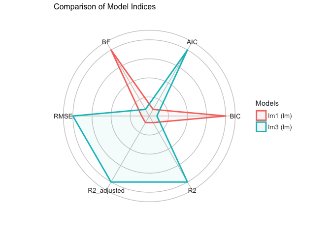
5. Conclusion
This analysis leads us to fail to reject the hypothesis according which a combination of both REDD+ project-based support and governance indicators increase would have a higher correlation with a decrease of deforestation rate. REDD+ advancement itself does not bear sufficient explanatory power, but without REDD+, a country development process does not lead to a decrease in the deforestation rate. This conclusion reinforces the idea that the double strategy of REDD+ makes sense: international organizations’ support should go both to projects and development policies. However, because this was an introductory analysis to the subject, and because of technical issues met here, this research would benefit from more research. It would be interesting, for instance, to study how deforestation has been evolving throughout time, and to add variables related to conflicts (as deforestation is affected by many variables and as the outliers - Burundi, Philippines -, may lead to think), in order to be certain of the relationship we are studying. It may also be interesting, in further studies, to focus on geographical tendencies, differentiating between Africa, Latin America and Asia, or even by forest basin, as the deforestation rates and drivers differ a lot in between the Congo Basin and the Amazon for instance.
Co-Director
Global Governance Centre
Professor
International Relations and Political Science
President
Global Governance Research Centre Consortium
International institutions and political networks.