Carolina Fontes
1. Introduction
Women’s access to land, both regarding its use and control, has been limited and restricted throughout the world. Gender inequality in accessing productive and financial resources, including land’s rights properties, are related to a large extent to women’s economic, social and cultural exclusion in society. Challenges to women’s use and control over land as well as to other productive resources have been often attributed to insufficient legal provisions, ineffective implementation of these laws and to discriminatory cultural practices inside a community (UN Women, 2013).
Despite a growing number of literature on women’s land rights (Jacobs, 2013; Deere and León, 2001; Agarwal, 1994), the causes of such a gendered structure regarding a secure access to land assets in practice has been less explored. Most studies relate women’s restricted de facto control and use of land in practice to a deficiency in countries legislation. In many countries, constitutional rights to assure gender equality in access to land are observed, nevertheless, these rights are contradicted by laws in the matter of marriage, divorce and inheritance that discriminate women and daughters. Lack of implementation of existing laws and secure protection to women against land grabbing and legal struggles are also pointed as main restrictions factors (Sida, 2012).
Although few works have paid attention to how customary, traditional and social practices as well as power gendered structures affect directly women’s secure access to land assets de facto, specific types of discrimination exercised by within these practices have been less examined.
This paper seeks to look to discrimination in the family as one of the types of discrimination that has an important impact on women’s use and control of land in practice. Discrimination in the family, understood as the primary source of discrimination girls face, will be considered therefore as the main channel of traditional and social practices that directly affect women’s secure access to land assets de facto.
The research question that this paper will seek to answer is: Does discrimination in the family affect women’s secure access to land assets in practice? The hypothesis that it will seek to verify is that discrimination in the family does affect a secure access to land in practice, as it is the first source of discrimination, of a power gendered social and economic structure, and main mechanism of traditional and social practices that reinforces women inequal access to land.
library(tidyverse)
library(knitr)
library(readxl)
library(ggplot2)
library(sjPlot)
library(stargazer)
library(olsrr)
library(gridExtra)
library(table1)
library(forecast)
library(ggcorrplot)
library(tseries)
library(lmtest)
library(pscl)
library(car)
library(outliers)
library(lindia)
library(ggfortify)
library(lawstat)

# setwd("C:/Users/Carolina Fontes/Documents/Documents/IHEID/Spring Semester. 2020/Stats II/Paper")

Data_4 <- read_excel("Data_4 . Carolina Fontes.xlsx")
2. Data
The data used in this report was collected on Land Portal database and the indicators of the Social Institutions and Gender Index 2019 (SIGI 2019) , provided by the Organization for Economic Cooperation and Development (OECD). The index measure of the variables chose here were calculated by the SIGI 2019. It explores gender discrimination regarding land ownership and in agriculture in 180 countries.
The dependent variable is secure access to land assets in practice (PRACTICElandacc), expressed as “a percentage of women among the total number of agriculture holders” (OECD, 2019). The agricultural holder is understood as the civil or juridical person in charge of the main decisions on use and management control over the agricultural holding resource, or in other words the economic agricultural land. This variable considers, therefore, land used for production purposes, without regard to title in legal form, and measures the incidence of women among agricultural holders.
The main predictor is discrimination in the family (Discrfamily), which includes consideration to formal and informal laws, economic, social, cultural norms and practices that coexist with the legislation system, with customary law, religious rules, embracing parental authority, marriage, household responsibilities, divorce and inheritance rights. This variable “captures social institutions that limit women’s decision-making power and undervalues their status in the household and the family” (Land Portal) . The measurement unit is expressed in percentage of discriminated women in the family in the country.
This work will control for the variables a) restricted civil liberties (civilliberties), which “captures discriminatory laws and practices that restrict women’s access to public space, their political voice and their participation in all aspects of public life” (Land Portal). This variable is measured in percentage of restricted civil liberties of women; b) restricted physical integrity (physicalintegrity), understood as “social institutions that limit women’s and girls’ control over their bodies, that increase women’s vulnerability, and that normalize attitudes toward gender-based violence” (Land Portal), with the measurement unit in in expressed in percentage; c) restricted access to productive and financial resources (financialresources), which captures “women’s restricted access to and control over critical productive and economic resources and assets” (Land Portal), also measured in percentage; d) Secure access to land assets guaranteed by law (LAWlandacc), was expressed as categorical variable, ranging from 0, 0.25, 0.5, 0.75 to 1 (being 0 the best legal framework on equal access rights and 1 no equal legal rights between women and men on access to land ownership); and e) SIGI 2019 (SIGI2019), the Index calculated by the development center of the OECD, and that takes into consideration the indicators and variables above. The measurement unit is an index ranging from 0 to 100, as lower values indicate lower levels of discrimination in social institutions, and the SIGI ranges from 0% for no discrimination to 100% for very high discrimination.
Although this data counts with a large number of missing values, this report opted not to include these missing values by omitting NAs. It proceeded in this way, since it considers that all the classes to be predicted are sufficiently represented by the data and that sufficient observations were included, so that the model does not lose statistical power.
Data <- na.omit(Data_4)

Data$PRACTICElandacc<- as.numeric(as.character(Data$PRACTICElandacc))

Data$Discrfamily<- as.numeric(as.character(Data$Discrfamily))

Data$financialresources<- as.numeric(as.character(Data$financialresources))

Data$civilliberties<- as.numeric(as.character(Data$civilliberties))

Data$physicalintegrity<- as.numeric(as.character(Data$physicalintegrity))

Data$SIGI2019<- as.numeric(as.character(Data$SIGI2019))

Data$LAWlandacc <- factor(Data$LAWlandacc)
Descriptive statistics of the data can be verified below.
table1(~PRACTICElandacc+Discrfamily+financialresources+civilliberties+physicalintegrity+SIGI2019, Data)
[1] "
| Overall (N=67) | |
|---|---|
| PRACTICElandacc | |
| Mean (SD) | 18.2 (8.91) |
| Median \[Min, Max\] | 15.4 \[3.10, 36.3\] |
| Discrfamily | |
| Mean (SD) | 34.2 (16.0) |
| Median \[Min, Max\] | 28.0 \[0.100, 87.7\] |
| financialresources | |
| Mean (SD) | 22.6 (15.6) |
| Median \[Min, Max\] | 19.8 \[2.10, 67.2\] |
| civilliberties | |
| Mean (SD) | 25.1 (15.3) |
| Median \[Min, Max\] | 21.2 \[5.30, 62.1\] |
| physicalintegrity | |
| Mean (SD) | 19.7 (10.6) |
| Median \[Min, Max\] | 18.1 \[4.20, 56.9\] |
| SIGI2019 | |
| Mean (SD) | 25.8 (12.1) |
| Median \[Min, Max\] | 23.2 \[8.10, 56.7\] |
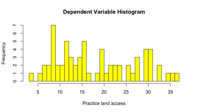
The distribution of the dependent variable can be visualized by the histogram below. It is skewed to the right, indicating that most frequently throughout the countries analyzed women represent low percentage of agricultural holders among the total land holders.
hist(Data$PRACTICElandacc, breaks=30, col="yellow", xlab="Practice land access", main="Dependent Variable Histogram")
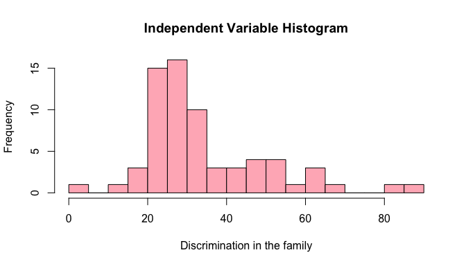
The distribution of the main independent variable can be visualized by the histogram below. It is also skewed to the right, in this case meaning that the countries where discrimination in the family achieve extreme percentage are not the majority.
hist(Data$Discrfamily, breaks=30, col="lightpink", xlab="Discrimination in the family", main="Independent Variable Histogram")
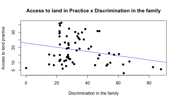
In the scatter plot below, we can observe the relationship between the dependent variable and the main independent variable as well as perceive its linearity. There seems to be a linear relationship between women’s secure access to land in practice and discrimination in the family. The association is also negative, indicating that as discrimination in the family increases, the percentage of women with access to control over the agricultural holding resource decreases.
attach(Data)

plot(Discrfamily, PRACTICElandacc, main="Access to land in Practice x Discrimination in the family",
   xlab="Discrimination in the family", ylab="Access to land practice", pch=19, col="black") + abline(lm(PRACTICElandacc~Discrfamily), col="blue")
 integer(0)
3. Methods
vThe statistical method chosen was ordinary least squares (OLS) regression to estimate the linear relationship between the dependent variable and independent variable, premising the existence of a negative linear relationship between access to land assets in practice and the main predictor discrimination in the family.
In model lm1, only the dependent variable and main predictor were included. Discrimination in the family has a significant negative effect on land access in practice, confirming expectations.
lm1 <- lm(PRACTICElandacc ~ Discrfamily, data = Data)
lm1
Call: lm(formula = PRACTICElandacc ~ Discrfamily, data = Data)
Coefficients: (Intercept) Discrfamily
22.96 -0.14
summary(lm1)
Call: lm(formula = PRACTICElandacc ~ Discrfamily, data = Data)
Residuals: Min 1Q Median 3Q Max -16.4498 -6.5959 -0.2587 7.4934 16.5556
Coefficients: Estimate Std. Error t value Pr(>|t|)
(Intercept) 22.96375 2.51599 9.127 2.96e-13 *** Discrfamily -0.13997
0.06669 -2.099 0.0397 *
— Signif. codes: 0 ‘’ 0.001 ’’ 0.01 ’’ 0.05 ‘.’ 0.1 ’ ’ 1
Residual standard error: 8.688 on 65 degrees of freedom Multiple R-squared: 0.06347, Adjusted R-squared: 0.04906 F-statistic: 4.405 on 1 and 65 DF, p-value: 0.03972
tab_model(lm1)
| PRACTICElandacc | |||
|---|---|---|---|
| Predictors | Estimates | CI | p |
| (Intercept) | 22.96 | 17.94 – 27.99 | <0.001 |
| Discrfamily | -0.14 | -0.27 – -0.01 | 0.040 |
| Observations | 67 | ||
| R2 / R2 adjusted | 0.063 / 0.049 | ||
Model lm2 included the variables restricted access to productive and financial resources (financialresources), restricted civil liberties (civilliberties), and restricted physical integrity (physicalintegrity) as controls. Controlling for these variables, the negative effect of discrimination in family was reduced and turned out to be not significant anymore.
lm2 <- lm(PRACTICElandacc ~ Discrfamily+financialresources+civilliberties+physicalintegrity, data = Data)
lm2
Call: lm(formula = PRACTICElandacc ~ Discrfamily + financialresources + civilliberties + physicalintegrity, data = Data)
Coefficients: (Intercept) Discrfamily financialresources
civilliberties
24.28462 -0.07103 0.07818 0.02335
physicalintegrity
-0.30674
summary(lm2)
Call: lm(formula = PRACTICElandacc ~ Discrfamily + financialresources + civilliberties + physicalintegrity, data = Data)
Residuals: Min 1Q Median 3Q Max -14.780 -6.910 -1.862 6.469 17.332
Coefficients: Estimate Std. Error t value Pr(>|t|)
(Intercept) 24.28462 2.57821 9.419 1.43e-13 *** Discrfamily -0.07103
0.10276 -0.691 0.4920
financialresources 0.07818 0.08881 0.880 0.3821
civilliberties 0.02335 0.08894 0.263 0.7938
physicalintegrity -0.30674 0.13272 -2.311 0.0242 *
— Signif. codes: 0 ‘’ 0.001 ’’ 0.01 ’’ 0.05 ‘.’ 0.1 ’ ’ 1
Residual standard error: 8.524 on 62 degrees of freedom Multiple R-squared: 0.1403, Adjusted R-squared: 0.08479 F-statistic: 2.529 on 4 and 62 DF, p-value: 0.04939
tab_model(lm2)
| PRACTICElandacc | |||
|---|---|---|---|
| Predictors | Estimates | CI | p |
| (Intercept) | 24.28 | 19.13 – 29.44 | <0.001 |
| Discrfamily | -0.07 | -0.28 – 0.13 | 0.492 |
| financialresources | 0.08 | -0.10 – 0.26 | 0.382 |
| civilliberties | 0.02 | -0.15 – 0.20 | 0.794 |
| physicalintegrity | -0.31 | -0.57 – -0.04 | 0.024 |
| Observations | 67 | ||
| R2 / R2 adjusted | 0.140 / 0.085 | ||
In model lm3, the categorical variable access to land guaranteed by law (LAWlandacc) was added as control. Discrimination in the family remained insignificant as lm2, so did the categories of the added control variable.
lm3 <- lm(PRACTICElandacc ~ Discrfamily+financialresources+civilliberties+physicalintegrity+LAWlandacc, data = Data)
lm3
Call: lm(formula = PRACTICElandacc ~ Discrfamily + financialresources + civilliberties + physicalintegrity + LAWlandacc, data = Data)
Coefficients: (Intercept) Discrfamily financialresources
civilliberties
23.17373 -0.02606 0.02481 0.05440
physicalintegrity LAWlandacc0.25 LAWlandacc0.5 LAWlandacc0.75
-0.34428 1.71397 -3.59532 11.63622
LAWlandacc1
-1.26214
summary(lm3)
Call: lm(formula = PRACTICElandacc ~ Discrfamily + financialresources + civilliberties + physicalintegrity + LAWlandacc, data = Data)
Residuals: Min 1Q Median 3Q Max -13.756 -5.903 -2.582 6.059 17.189
Coefficients: Estimate Std. Error t value Pr(>|t|)
(Intercept) 23.17373 2.72431 8.506 8.73e-12 *** Discrfamily -0.02606
0.10791 -0.241 0.810
financialresources 0.02481 0.13809 0.180 0.858
civilliberties 0.05440 0.09441 0.576 0.567
physicalintegrity -0.34428 0.14145 -2.434 0.018 *
LAWlandacc0.25 1.71397 3.08872 0.555 0.581
LAWlandacc0.5 -3.59532 5.57748 -0.645 0.522
LAWlandacc0.75 11.63622 11.44247 1.017 0.313
LAWlandacc1 -1.26214 9.26635 -0.136 0.892
— Signif. codes: 0 ‘’ 0.001 ’’ 0.01 ’’ 0.05 ‘.’ 0.1 ’ ’ 1
Residual standard error: 8.594 on 58 degrees of freedom Multiple R-squared: 0.1824, Adjusted R-squared: 0.06966 F-statistic: 1.618 on 8 and 58 DF, p-value: 0.1396
tab_model(lm3)
| PRACTICElandacc | |||
|---|---|---|---|
| Predictors | Estimates | CI | p |
| (Intercept) | 23.17 | 17.72 – 28.63 | <0.001 |
| Discrfamily | -0.03 | -0.24 – 0.19 | 0.810 |
| financialresources | 0.02 | -0.25 – 0.30 | 0.858 |
| civilliberties | 0.05 | -0.13 – 0.24 | 0.567 |
| physicalintegrity | -0.34 | -0.63 – -0.06 | 0.018 |
| LAWlandacc \[0.25\] | 1.71 | -4.47 – 7.90 | 0.581 |
| LAWlandacc \[0.5\] | -3.60 | -14.76 – 7.57 | 0.522 |
| LAWlandacc \[0.75\] | 11.64 | -11.27 – 34.54 | 0.313 |
| LAWlandacc \[1\] | -1.26 | -19.81 – 17.29 | 0.892 |
| Observations | 67 | ||
| R2 / R2 adjusted | 0.182 / 0.070 | ||
Model lm4 controlled for restricted physical integrity (physicalintegrity) and access to land guaranteed by law (LAWlandacc). In this scenario, the effect of the main predictor became slightly positive.
lm4 <- lm(PRACTICElandacc ~ Discrfamily+physicalintegrity+LAWlandacc, data = Data)
lm4
Call: lm(formula = PRACTICElandacc ~ Discrfamily + physicalintegrity + LAWlandacc, data = Data)
Coefficients: (Intercept) Discrfamily physicalintegrity LAWlandacc0.25
23.4653428 0.0006535 -0.3281938 2.2400538
LAWlandacc0.5 LAWlandacc0.75 LAWlandacc1
-2.3615717 12.5809128 -0.1091316
summary(lm4)
Call: lm(formula = PRACTICElandacc ~ Discrfamily + physicalintegrity + LAWlandacc, data = Data)
Residuals: Min 1Q Median 3Q Max -13.143 -5.796 -2.246 5.927 16.988
Coefficients: Estimate Std. Error t value Pr(>|t|)
(Intercept) 23.4653428 2.6507320 8.852 1.75e-12 *** Discrfamily
0.0006535 0.0980750 0.007 0.9947
physicalintegrity -0.3281938 0.1357396 -2.418 0.0187 *
LAWlandacc0.25 2.2400538 2.5443441 0.880 0.3822
LAWlandacc0.5 -2.3615717 4.8320221 -0.489 0.6268
LAWlandacc0.75 12.5809128 8.7032213 1.446 0.1535
LAWlandacc1 -0.1091316 6.8983571 -0.016 0.9874
— Signif. codes: 0 ‘’ 0.001 ’’ 0.01 ’’ 0.05 ‘.’ 0.1 ’ ’ 1
Residual standard error: 8.48 on 60 degrees of freedom Multiple R-squared: 0.1765, Adjusted R-squared: 0.09418 F-statistic: 2.144 on 6 and 60 DF, p-value: 0.06127
tab_model(lm4)
| PRACTICElandacc | |||
|---|---|---|---|
| Predictors | Estimates | CI | p |
| (Intercept) | 23.47 | 18.16 – 28.77 | <0.001 |
| Discrfamily | 0.00 | -0.20 – 0.20 | 0.995 |
| physicalintegrity | -0.33 | -0.60 – -0.06 | 0.019 |
| LAWlandacc \[0.25\] | 2.24 | -2.85 – 7.33 | 0.382 |
| LAWlandacc \[0.5\] | -2.36 | -12.03 – 7.30 | 0.627 |
| LAWlandacc \[0.75\] | 12.58 | -4.83 – 29.99 | 0.154 |
| LAWlandacc \[1\] | -0.11 | -13.91 – 13.69 | 0.987 |
| Observations | 67 | ||
| R2 / R2 adjusted | 0.177 / 0.094 | ||
Model lm5 controlled just for physical integrity (physicalintegrity). Discrimination in family remained with its negative effect, although not significant.
lm5 <- lm(PRACTICElandacc ~ Discrfamily+physicalintegrity, data = Data)
lm5
Call: lm(formula = PRACTICElandacc ~ Discrfamily + physicalintegrity, data = Data)
Coefficients: (Intercept) Discrfamily physicalintegrity
24.38749 -0.02235 -0.27687
summary(lm5)
Call: lm(formula = PRACTICElandacc ~ Discrfamily + physicalintegrity, data = Data)
Residuals: Min 1Q Median 3Q Max -14.203 -6.645 -1.914 6.795 15.943
Coefficients: Estimate Std. Error t value Pr(>|t|)
(Intercept) 24.38749 2.53429 9.623 4.69e-14 *** Discrfamily -0.02235
0.08461 -0.264 0.7925
physicalintegrity -0.27687 0.12787 -2.165 0.0341 *
— Signif. codes: 0 ‘’ 0.001 ’’ 0.01 ’’ 0.05 ‘.’ 0.1 ’ ’ 1
Residual standard error: 8.452 on 64 degrees of freedom Multiple R-squared: 0.1274, Adjusted R-squared: 0.1001 F-statistic: 4.672 on 2 and 64 DF, p-value: 0.01277
tab_model(lm5)
| PRACTICElandacc | |||
|---|---|---|---|
| Predictors | Estimates | CI | p |
| (Intercept) | 24.39 | 19.32 – 29.45 | <0.001 |
| Discrfamily | -0.02 | -0.19 – 0.15 | 0.793 |
| physicalintegrity | -0.28 | -0.53 – -0.02 | 0.034 |
| Observations | 67 | ||
| R2 / R2 adjusted | 0.127 / 0.100 | ||
Nevertheless, this was the model chosen not even because it has the highest adjusted R squared and the smallest AIC, but also for theoretical reasons, as it will be explained later.
stargazer(lm1, lm2, lm3, lm4, lm5,
          title = "Secure access to land in practice",
          type = "text")
Secure access to land in practice
                                                         Dependent variable:
                -----------------------------------------------------------------------------------------------------
                                                           PRACTICElandacc
                        (1)                  (2)                 (3)                 (4)                 (5)
| Discrfamily -0.140** -0.071 -0.026 0.001 -0.022 (0.067) (0.103) (0.108) (0.098) (0.085) |
| financialresources 0.078 0.025 (0.089) (0.138) |
| civilliberties 0.023 0.054 (0.089) (0.094) |
| physicalintegrity -0.307** -0.344** -0.328** -0.277** (0.133) (0.141) (0.136) (0.128) |
| LAWlandacc0.25 1.714 2.240 (3.089) (2.544) |
| LAWlandacc0.5 -3.595 -2.362 (5.577) (4.832) |
| LAWlandacc0.75 11.636 12.581 (11.442) (8.703) |
| LAWlandacc1 -1.262 -0.109 (9.266) (6.898) |
| Constant 22.964*** 24.285*** 23.174*** 23.465*** 24.387*** (2.516) (2.578) (2.724) (2.651) (2.534) |
{\normalsize Observations 67 67 67 67 67
R2 0.063 0.140 0.182 0.177 0.127
Adjusted R2 0.049 0.085 0.070 0.094 0.100
Residual Std. Error 8.688 (df = 65) 8.524 (df = 62) 8.594 (df = 58)
8.480 (df = 60) 8.452 (df = 64)
F Statistic 4.405** (df = 1; 65) 2.529** (df = 4; 62) 1.618 (df = 8;
58) 2.144* (df = 6; 60) 4.672** (df = 2; 64)}
Note: *p<0.1; **p<0.05; ***p<0.01
tab_model(lm1, lm2, lm3, lm4, lm5, show.aic = TRUE)
| PRACTICElandacc | PRACTICElandacc | PRACTICElandacc | PRACTICElandacc | PRACTICElandacc | |||||||||||
|---|---|---|---|---|---|---|---|---|---|---|---|---|---|---|---|
| Predictors | Estimates | CI | p | Estimates | CI | p | Estimates | CI | p | Estimates | CI | p | Estimates | CI | p |
| (Intercept) | 22.96 | 17.94 – 27.99 | <0.001 | 24.28 | 19.13 – 29.44 | <0.001 | 23.17 | 17.72 – 28.63 | <0.001 | 23.47 | 18.16 – 28.77 | <0.001 | 24.39 | 19.32 – 29.45 | <0.001 |
| Discrfamily | -0.14 | -0.27 – -0.01 | 0.040 | -0.07 | -0.28 – 0.13 | 0.492 | -0.03 | -0.24 – 0.19 | 0.810 | 0.00 | -0.20 – 0.20 | 0.995 | -0.02 | -0.19 – 0.15 | 0.793 |
| financialresources | 0.08 | -0.10 – 0.26 | 0.382 | 0.02 | -0.25 – 0.30 | 0.858 | |||||||||
| civilliberties | 0.02 | -0.15 – 0.20 | 0.794 | 0.05 | -0.13 – 0.24 | 0.567 | |||||||||
| physicalintegrity | -0.31 | -0.57 – -0.04 | 0.024 | -0.34 | -0.63 – -0.06 | 0.018 | -0.33 | -0.60 – -0.06 | 0.019 | -0.28 | -0.53 – -0.02 | 0.034 | |||
| LAWlandacc \[0.25\] | 1.71 | -4.47 – 7.90 | 0.581 | 2.24 | -2.85 – 7.33 | 0.382 | |||||||||
| LAWlandacc \[0.5\] | -3.60 | -14.76 – 7.57 | 0.522 | -2.36 | -12.03 – 7.30 | 0.627 | |||||||||
| LAWlandacc \[0.75\] | 11.64 | -11.27 – 34.54 | 0.313 | 12.58 | -4.83 – 29.99 | 0.154 | |||||||||
| LAWlandacc \[1\] | -1.26 | -19.81 – 17.29 | 0.892 | -0.11 | -13.91 – 13.69 | 0.987 | |||||||||
| Observations | 67 | 67 | 67 | 67 | 67 | ||||||||||
| R2 / R2 adjusted | 0.063 / 0.049 | 0.140 / 0.085 | 0.182 / 0.070 | 0.177 / 0.094 | 0.127 / 0.100 | ||||||||||
| AIC | 483.814 | 484.082 | 488.712 | 485.194 | 481.077 | ||||||||||
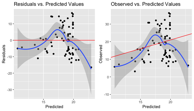
When checking assumptions, doubts emerged regarding the linearity verified through residuals vs predicted values and observed vs predicted values plots. Points look like somewhat symmetrically distributed, but at the same time, a small bow can be observed.
plotpreds <- function(lm5, data = Data){
p1 <- ggplot(lm5, aes(.fitted, .resid)) +
  geom_point() +
  stat_smooth(method="loess") +
  geom_hline(yintercept=0, col="red") +
  xlab("Predicted") + ylab("Residuals") +
  ggtitle("Residuals vs. Predicted Values")
df_plt <- data.frame("fitted" = fitted(lm5),
                  "observed" = Data$PRACTICElandacc)
p2 <- ggplot(df_plt, aes(x=fitted, y=observed)) +
  geom_point() + stat_smooth(method="loess") +
  geom_abline(intercept = 1, col="red") +
  xlab("Predicted") + ylab("Observed") +
  ggtitle("Observed vs. Predicted Values")
grid.arrange(p1, p2, ncol=2)
}

landacc <- lm(PRACTICElandacc ~ Discrfamily, Data)

plotpreds(landacc, Data)

As a robustness check, squaring the main predictor, most common way to deal with nonlinearity, did not change much this pattern. In this case, this report takes into consideration that the relationship between dependent variable and independent variables plus the error term is to a great extension linear.
Discrfamily2 <- lm(PRACTICElandacc ~ physicalintegrity +
                I(Discrfamily^2), Data)

summary(Discrfamily2)
Call: lm(formula = PRACTICElandacc ~ physicalintegrity + I(Discrfamily^2), data = Data)
Residuals: Min 1Q Median 3Q Max -14.469 -6.417 -1.059 6.207 15.745
Coefficients: Estimate Std. Error t value Pr(>|t|)
(Intercept) 23.7641641 2.1827713 10.887 3.33e-16 ***
physicalintegrity -0.2101385 0.1252210 -1.678 0.0982 .
I(Discrfamily^2) -0.0010216 0.0009129 -1.119 0.2673
— Signif. codes: 0 ‘’ 0.001 ’’ 0.01 ’’ 0.05 ‘.’ 0.1 ’ ’ 1
Residual standard error: 8.375 on 64 degrees of freedom Multiple R-squared: 0.1432, Adjusted R-squared: 0.1164 F-statistic: 5.348 on 2 and 64 DF, p-value: 0.007113
plotpreds <- function(Discrfamily2, data = Data){
p1 <- ggplot(Discrfamily2, aes(.fitted, .resid)) +
  geom_point() +
  stat_smooth(method="loess") +
  geom_hline(yintercept=0, col="red") +
  xlab("Predicted") + ylab("Residuals") +
  ggtitle("Residuals vs. Predicted Values")
df_plt <- data.frame("fitted" = fitted(Discrfamily2),
                  "observed" = Data$PRACTICElandacc)
p2 <- ggplot(df_plt, aes(x=fitted, y=observed)) +
  geom_point() + stat_smooth(method="loess") +
  geom_abline(intercept = 1, col="red") +
  xlab("Predicted") + ylab("Observed") +
  ggtitle("Observed vs. Predicted Values")
grid.arrange(p1, p2, ncol=2)
}

landacc2 <- lm(PRACTICElandacc ~ Discrfamily^2, Data)

plotpreds(landacc2, Data)
Multicollinearity was checked through the calculation of high variance inflation factors (VIFs). There seems not to be a problem in this case, as values are close to 1.
vif(lm5)

  Discrfamily physicalintegrity
     1.701102          1.701102

t(t(vif(lm5)))

                  [,1]
Discrfamily 1.701102 physicalintegrity 1.701102
## no multicollinearity
Checking for endogeneity, we fail to reject the null hypothesis that gama is zero, meaning that there are no signs of misspecification, particularly nonlinearity.
resettest(lm5, type = "fitted")

RESET test
data: lm5 RESET = 0.19641, df1 = 2, df2 = 62, p-value = 0.8222
Testing correlations between independent variables and residuals with the Person correlation test demonstrated that there is no evidence of correlation.
cor.test(Data$Discrfamily, lm5$residuals)

Pearson's product-moment correlation
data: DataDiscrfamilyandl**m5residuals t = -2.053e-17, df = 65, p-value = 1 alternative hypothesis: true correlation is not equal to 0 95 percent confidence interval: -0.2402086 0.2402086 sample estimates: cor -2.546484e-18
cor.test(Data$physicalintegrity, lm5$residuals)

Pearson's product-moment correlation
data: Dataphysicalintegrityandl**m5residuals t = -2.5546e-16, df = 65, p-value = 1 alternative hypothesis: true correlation is not equal to 0 95 percent confidence interval: -0.2402086 0.2402086 sample estimates: cor -3.168551e-17
To diagnose autocorrelation, it was used the autocorrelation function (ACF) plot, by which we can see that there is not really a trend for autocorrelation.
ggAcf(lm5$residuals)
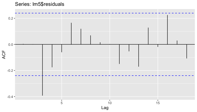
When considering the Wald-Wolfowitz runs test, we fail to reject the null hypothesis that there are random runs or sequences and, therefore, assume that the residuals are not autocorrelated.
runs.test(lm5$residuals)

Runs Test - Two sided
data: lm5$residuals Standardized Runs Statistic = 0.12497, p-value = 0.9005
Regarding diagnosing normality, the assumption related to it that the error term should have a population mean of zero is respected, since the mean in this case is very close to zero.
mean(lm5$residuals)
[1] -3.299049e-16
## The mean is very close to zero
The normality probability (QQ) plot appears to have a s-shape pattern, so further tests were conducted to verify whether normality can be diagnosed.
df_resid <- data.frame(resid = lm5$residuals)
p <- ggplot(df_resid, aes(sample = resid))
p + stat_qq() + stat_qq_line()
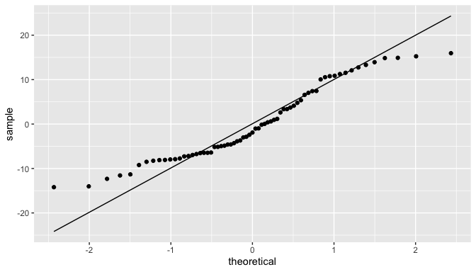
Although some tests used to test whether the residuals were normally distributed, particularly the Shapiro-Wilk test, presented a P-value below 0.05, meaning that the null hypothesis that the residuals are normally distributed would be rejected, this report will take into consideration the Jarque-Bera test. Even if it is not recognized as the most powerful normality test, for the purposes and objectives of this research report, it was considered enough to assume that the errors are normally distributed, as with the Jarque-Bera test we fail to reject the null hypothesis that skewness is zero and the excess of kurtosis is also zero.
ols_test_normality(lm5)
| Test Statistic pvalue |
|---|
| Shapiro-Wilk 0.9421 0.0037 Kolmogorov-Smirnov 0.1193 0.2735 Cramer-von Mises 5.4782 0.0000 Anderson-Darling 1.3492 0.0016 |
jarque.bera.test(lm5$residuals)

Jarque Bera Test
data: lm5$residuals X-squared = 4.367, df = 2, p-value = 0.1126
## normally distributed
When checking the assumption that the error term has equal variance, which would satisfy the condition of homoscedasticity, the residuals plot seems to suggest that the residuals grow as a function of fitted values, forming a cone shape and indicating that there is heteroskedasticity.
autoplot(lm5, which = c(1,3))
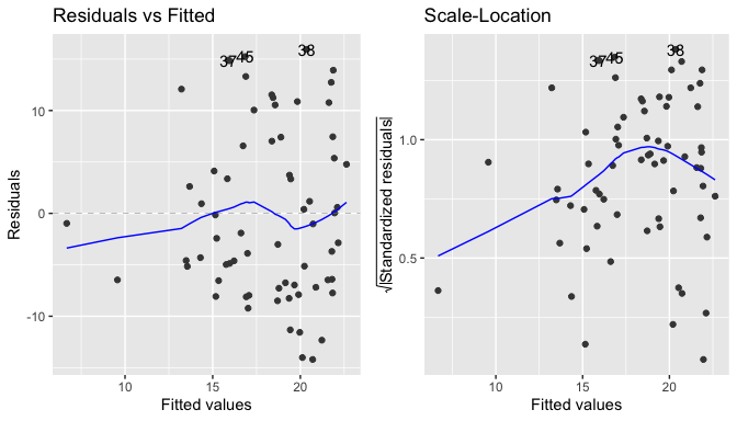
Nevertheless, when running the Breusch-Pagan test, the null hypothesis that the variance of the residuals is homogenous is not rejected, as the P-value is greater than 0.05. The condition of homoscedasticity, therefore, can be accepted.
bptest(lm5, data = Data, studentize = TRUE)

studentized Breusch-Pagan test
data: lm5 BP = 3.2227, df = 2, p-value = 0.1996
## With bptest, condition of homoskedasticity is satisfied
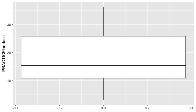
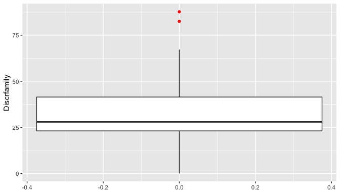
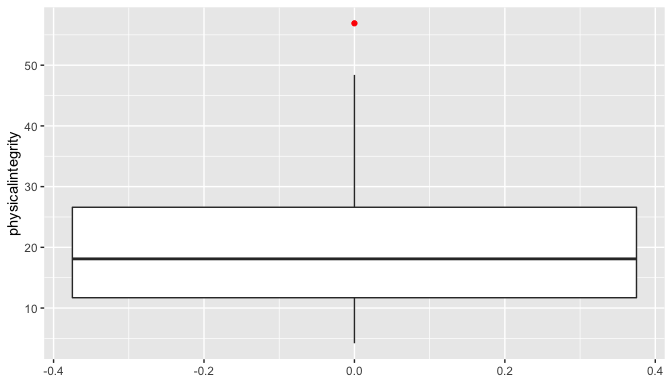
Outliers were identified as it can be observed in the box plots.
outlier(Data$PRACTICElandacc)
[1] 36.3
outlier(Data$PRACTICElandacc, opposite = TRUE)
[1] 3.1
ggplot(Data, aes(y = PRACTICElandacc)) +
  geom_boxplot(outlier.colour = "red")
ggplot(Data, aes(y = Discrfamily)) +
  geom_boxplot(outlier.colour = "red")
ggplot(Data, aes(y = physicalintegrity)) +
  geom_boxplot(outlier.colour = "red")
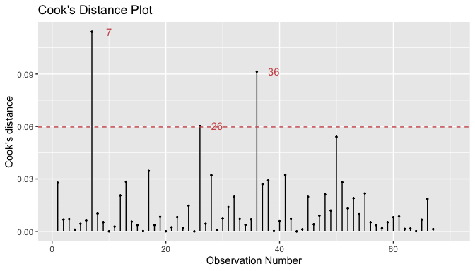
The Cook’s Distance plot shows which observations would impact this specific chosen regression model if they were deleted, due to their influence on the predicted outcome. The points with high Cook’s D are 7 (Antigua and Barbuda), 26 (Bhutan) and 36 (Congo).
gg_cooksd(lm5)
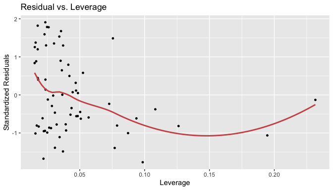
It is possible to observe as well by the dfbeta diagnostic that these observations are the ones that have a higher leverage and a big residual.
gg_resleverage(lm5)
ols_plot_dfbetas(lm5)
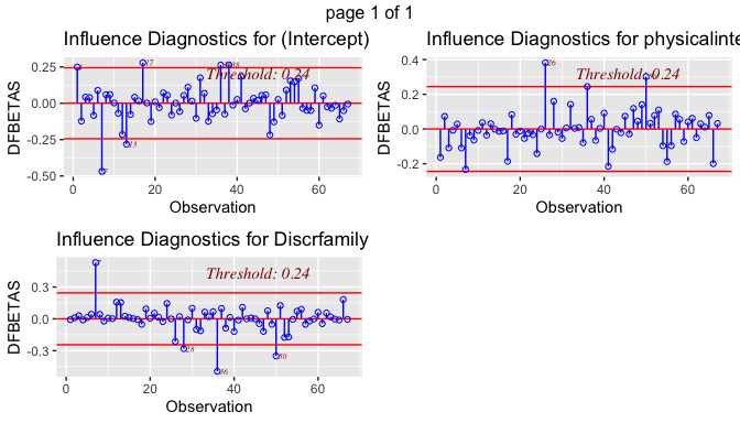
However, as a robustness check, running the model without these observations demonstrated that there were no meaningful changes, once the signs and significance remained the same with no major changes in the coefficient effects. The outliers were, therefore, kept in the model.
Data2 <- Data[-c(7,26,36),]

lm6 <- lm(PRACTICElandacc ~ Discrfamily + physicalintegrity, Data2)

tab_model(lm5, lm6, dv.labels = c("With Outliers","Without Outliers"))
| With Outliers | Without Outliers | |||||
|---|---|---|---|---|---|---|
| Predictors | Estimates | CI | p | Estimates | CI | p |
| (Intercept) | 24.39 | 19.32 – 29.45 | <0.001 | 25.01 | 19.72 – 30.31 | <0.001 |
| Discrfamily | -0.02 | -0.19 – 0.15 | 0.793 | -0.01 | -0.20 – 0.18 | 0.926 |
| physicalintegrity | -0.28 | -0.53 – -0.02 | 0.034 | -0.32 | -0.59 – -0.06 | 0.018 |
| Observations | 67 | 64 | ||||
| R2 / R2 adjusted | 0.127 / 0.100 | 0.158 / 0.130 | ||||
To a great extent, it was demonstrated that the OLS assumptions were satisfied, therefore, respecting the Gauss-Markov Theorem, which states that the OLS is the BLUE – Best (minimizes variance), Linear, Unbiased (e(B) = B), Estimator – “of populations parameters if errors uncorrelated with equal variance and a mean of zero” (slides).
4. Results
As mentioned before, lm5 was the model chosen, although the main predictor, discrimination in the family, is not significant. In this model, the effect association of this main independent variable was negative as expected, since the women’s secure access to land in practice (expressed in percentage of women holding control over land) decreases as discrimination against women in the family increases.
Compared to the other fitted models used to check robustness (as per table below), this model was selected not only because it has the highest adjusted R squared and the smallest AIC, but also for theoretical reasons. It controlled for the variable restricted physical integrity (physicalintegrity). Controlling for restricted physical integrity was important, as vulnerability and control over a woman’s own body may affect the ability of a woman discriminated by the family to manage to control de facto over land assets, which is, in its turn, less explored by the literature.
tab_model(lm1, lm2, lm3, lm4, lm5, show.aic = TRUE)
| PRACTICElandacc | PRACTICElandacc | PRACTICElandacc | PRACTICElandacc | PRACTICElandacc | |||||||||||
|---|---|---|---|---|---|---|---|---|---|---|---|---|---|---|---|
| Predictors | Estimates | CI | p | Estimates | CI | p | Estimates | CI | p | Estimates | CI | p | Estimates | CI | p |
| (Intercept) | 22.96 | 17.94 – 27.99 | <0.001 | 24.28 | 19.13 – 29.44 | <0.001 | 23.17 | 17.72 – 28.63 | <0.001 | 23.47 | 18.16 – 28.77 | <0.001 | 24.39 | 19.32 – 29.45 | <0.001 |
| Discrfamily | -0.14 | -0.27 – -0.01 | 0.040 | -0.07 | -0.28 – 0.13 | 0.492 | -0.03 | -0.24 – 0.19 | 0.810 | 0.00 | -0.20 – 0.20 | 0.995 | -0.02 | -0.19 – 0.15 | 0.793 |
| financialresources | 0.08 | -0.10 – 0.26 | 0.382 | 0.02 | -0.25 – 0.30 | 0.858 | |||||||||
| civilliberties | 0.02 | -0.15 – 0.20 | 0.794 | 0.05 | -0.13 – 0.24 | 0.567 | |||||||||
| physicalintegrity | -0.31 | -0.57 – -0.04 | 0.024 | -0.34 | -0.63 – -0.06 | 0.018 | -0.33 | -0.60 – -0.06 | 0.019 | -0.28 | -0.53 – -0.02 | 0.034 | |||
| LAWlandacc \[0.25\] | 1.71 | -4.47 – 7.90 | 0.581 | 2.24 | -2.85 – 7.33 | 0.382 | |||||||||
| LAWlandacc \[0.5\] | -3.60 | -14.76 – 7.57 | 0.522 | -2.36 | -12.03 – 7.30 | 0.627 | |||||||||
| LAWlandacc \[0.75\] | 11.64 | -11.27 – 34.54 | 0.313 | 12.58 | -4.83 – 29.99 | 0.154 | |||||||||
| LAWlandacc \[1\] | -1.26 | -19.81 – 17.29 | 0.892 | -0.11 | -13.91 – 13.69 | 0.987 | |||||||||
| Observations | 67 | 67 | 67 | 67 | 67 | ||||||||||
| R2 / R2 adjusted | 0.063 / 0.049 | 0.140 / 0.085 | 0.182 / 0.070 | 0.177 / 0.094 | 0.127 / 0.100 | ||||||||||
| AIC | 483.814 | 484.082 | 488.712 | 485.194 | 481.077 | ||||||||||
With the anova test, it is possible to reject the null hypothesis that the increase in the model fit – the original model (lm1) by adding the variable restricted physical integrity – is zero, in favor of the alternative hypothesis that at least one independent variable has effect on women’s access to land in practice, confirming that the variable restricted physical integrity has an explanatory role in the model.
anova(lm1, lm5)
Analysis of Variance Table
Model 1: PRACTICElandacc ~ Discrfamily Model 2: PRACTICElandacc ~
Discrfamily + physicalintegrity Res.Df RSS Df Sum of Sq F Pr(>F)
1 65 4906.8
2 64 4571.8 1 334.92 4.6884 0.0341 * — Signif. codes: 0 ‘’ 0.001
’’ 0.01 ’’ 0.05 ‘.’ 0.1 ’ ’ 1
5. Conclusion
This report demonstrated that women’s secure access to land in practice is affected by discrimination of women and girls in the family, controlling for physical integrity.
The negative effect association shows that in countries where discrimination against women inside the family reflects a high percentage, the percentage of women detaining control and use of land assets decreases, confirming that gendered family structures impact women’s access to agriculture holdings de facto, reproducing gender socio-economic inequalities. Controlling for restricted physical integrity demonstrated that gender-based violence and women’s body vulnerability also has an impact in these variables association, constraining women’s secure access to land.
This report recognizes, nevertheless, its limitations. Better accounts of missing values and normality of the residuals’ distribution should be considered in the future, in order to improve the model presented in this study.
References:
Agarwal, B. (1994). A field of one’s own: women and land rights in South Asia. Cambridge: Cambridge University Press.
Deere, C. D., & Leôn, M. (2001). Empowering women: land and property rights in Latin America. Pittsburgh: Pittsburgh University Press.
Jacobs, S. (2013). Gender, Land and Sexuality: Exploring connections. International Journal of Politics, Culture, and Society, 27:2, 173-190.
Land Portal website. Social Institutions and Gender Index (2019). [online]. Available at: https://landportal.org/book/indicator/oecd-sigi2019sigi (Accessed: 14 April, 2020).
Organization for Economic Cooperation and Development (OECD). OECD Stat (2019). [online]. Available at: https://stats.oecd.org/Index.aspx?DataSetCode=GIDDB2019 (Accessed: 14 April, 2020).
Social Institutions and Gender Index (SIGI). SIGI results 2019. [online]. Available at: https://www.genderindex.org/ranking/ (Accessed: 14 April, 2020).
Swedish International Development Cooperation Agency (Sida). Quick guide to what and how: increasing women’s access to land. [online]. Available at: https://www.oecd.org/dac/gender-development/47566053.pdf (Accessed: 19 May, 2020).
UN Women, 2013. Realizing women’s rights to land and other productive resources. UN Women handbook. [online]. Available at: https://www.unwomen.org/-/media/headquarters/attachments/sections/library/publications/2013/11/ohchr-unwomen-land-rights-handbook-web%20pdf.pdf?la=en&vs=1455 (Accessed: 19 May, 2020).
Co-Director
Global Governance Centre
Professor
International Relations and Political Science
President
Global Governance Research Centre Consortium
International institutions and political networks.