Trust in Whatsapp and Facebook: Speculations from India:Voters are divided across caste, and not across party preference
Vishnu Varatharajan - Statistics for International Relations Research II
- INTRODUCING THE DATASET
- DATASET INSPECTION AND CLEANING
- VARIABLES AND THEORETICAL APPROACH
- REGRESSION
- DIAGNOSTICS
- CONCLUSION
Data: pooledthreeway_data.dta
**WARNING: THIS DOCUMENT DOES NOT WANT TO AUTOMATICALLY INSTALL RELEVANT PACKAGES ON YOUR COMPUTER WITHOUT PRIOR CONSENT, SO MAKE SURE THE FOLLOWING PACKAGES ARE INSTALLED FOR THE CODES TO PROPERLY FUNCTION.**
tidyverse
haven
car
sjPlot
survey
naniar
INTRODUCING THE DATASET
This dataset contains 112,272 100,000 observations and 104 variables, coding the three-way survey asking Indians about their political affiliations and personal details. This dataset was prepared to find whether digital media literacy intervention increases comprehension between mainstream news and false news in the United States and India. This project was involved in the creation of multiple datasets, and I have singled out a dataset that was created by pooling in all the data that was collected in India between 2018-2019. First, I shall import the dataset by entering the following command:
data_old <- read_dta("pooledthreeway_data.dta")
This dataset contains 104 variables out of which 21 interested me. Out of those 21, I singled out six variables that were relevant for my blogpost. Creating a new dataset using those variables,
data <- select(data_old, facebookaccuracy, whatsappaccuracy, BJP_feelings, INC_feelings, caste, political_interest)
DATASET INSPECTION AND CLEANING
Let me subject the dataset into a series of inspections.
Checking the structure of the dataset:
I intuitively know which variables are supposed to be numerical and which are to be categorical, but we need to make sure whether the structure of this dataset is intact:
str(data)

## tibble[,6] [112,272 × 6] (S3: tbl_df/tbl/data.frame)
##  $ facebookaccuracy  : num [1:112272] NA NA NA NA NA NA NA NA NA NA ...
##   ..- attr(*, "label")= chr "_71 if 1/4"
##   ..- attr(*, "format.stata")= chr "%9.0g"
##  $ whatsappaccuracy  : num [1:112272] NA NA NA NA NA NA NA NA NA NA ...
##   ..- attr(*, "label")= chr "_72 if 1/4"
##   ..- attr(*, "format.stata")= chr "%9.0g"
##  $ BJP_feelings      : num [1:112272] 3 3 3 3 3 3 3 3 3 3 ...
##   ..- attr(*, "format.stata")= chr "%9.0g"
##  $ INC_feelings      : num [1:112272] 3 3 3 3 3 3 3 3 3 3 ...
##   ..- attr(*, "format.stata")= chr "%9.0g"
##  $ caste             : num [1:112272] 1 1 1 1 1 1 1 1 1 1 ...
##   ..- attr(*, "label")= chr "q_137 if 1/5"
##   ..- attr(*, "format.stata")= chr "%9.0g"
##  $ political_interest: num [1:112272] 4 4 4 4 4 4 4 4 4 4 ...
##   ..- attr(*, "format.stata")= chr "%9.0g"
As expected, this dataset requires cleaning. the variables here are coded as numerical variables, but the variables that we deal with here are categorical variables, so we have some factoring work to do:
data$facebookaccuracy = factor(data$facebookaccuracy, levels = c(1,2,3,4), labels = c("Not at all accurate", "Not very accurate", "Somewhat accurate", "Very accurate"))
data$whatsappaccuracy = factor(data$whatsappaccuracy, levels = c(1,2,3,4), labels = c("Not at all accurate", "Not very accurate", "Somewhat accurate", "Very accurate"))
data$BJP_feelings = factor(data$BJP_feelings, levels = c(1,2,3,4), labels = c("Strongly dislike", "Somewhat dislike", "Somewhat like", "Strongly like"))
data$INC_feelings = factor(data$INC_feelings, levels = c(1,2,3,4), labels = c("Strongly dislike", "Somewhat dislike", "Somewhat like", "Strongly like"))
data$caste = factor(data$caste, levels = c(1,2,3,4,5), labels = c("SC", "ST", "OBC", "GEN", "Other"))
data$political_interest = factor(data$political_interest, levels = c(1,2,3,4,5), labels = c("Not at all interested", "Not very interested", "Somewhat interested", "Very interested", "Extremely interested"))
Now that we factored it, let’s check its structure again:
str(data)

## tibble[,6] [112,272 × 6] (S3: tbl_df/tbl/data.frame)
##  $ facebookaccuracy  : Factor w/ 4 levels "Not at all accurate",..: NA NA NA NA NA NA NA NA NA NA ...
##  $ whatsappaccuracy  : Factor w/ 4 levels "Not at all accurate",..: NA NA NA NA NA NA NA NA NA NA ...
##  $ BJP_feelings      : Factor w/ 4 levels "Strongly dislike",..: 3 3 3 3 3 3 3 3 3 3 ...
##  $ INC_feelings      : Factor w/ 4 levels "Strongly dislike",..: 3 3 3 3 3 3 3 3 3 3 ...
##  $ caste             : Factor w/ 5 levels "SC","ST","OBC",..: 1 1 1 1 1 1 1 1 1 1 ...
##  $ political_interest: Factor w/ 5 levels "Not at all interested",..: 4 4 4 4 4 4 4 4 4 4 ...
Perfect, I have factored the categorical variables accordingly.
Sample size of the dataset:
Let me check how many occurrences each variable has to make sure we have adequate number of samples to regress:
table(data$facebookaccuracy)

##
## Not at all accurate   Not very accurate   Somewhat accurate       Very accurate
##                3792               14752               26000                9184

table(data$whatsappaccuracy)

##
## Not at all accurate   Not very accurate   Somewhat accurate       Very accurate
##                4640               15792               25024                7664

table(data$BJP_feelings)

##
## Strongly dislike Somewhat dislike    Somewhat like    Strongly like
##            13104             6608            26432            56256

table(data$INC_feelings)

##
## Strongly dislike Somewhat dislike    Somewhat like    Strongly like
##            34208            14544            32864            16352

table(data$caste)

##
##    SC    ST   OBC   GEN Other
## 14848  3088 46688 42032  2464

table(data$political_interest)

##
## Not at all interested   Not very interested   Somewhat interested
##                 21216                  6912                 26480
##       Very interested  Extremely interested
##                 24048                 27728
We have adequate samples to work on our way.
Status of missing data
gg_miss_upset(data)
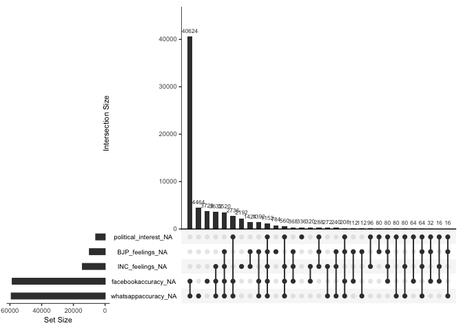
This graph is so refreshing to look at, because there are not so many missing values in our dataset compared to the sample size we have. We have huge missing values when facebookaccuracy and whatsapp accuracy are combines, but it it not a problem since they are separate dependent variables that I use in separate regressions.
Creating new binary variables:
In order to simplify the regression, I wish to convert the categorical variables as binary variables, and then proceed to introducing them:
data$facebook_binary <- recode(data$facebookaccuracy, "c('Not at all accurate','Not very accurate')='Not accurate';c('Somewhat accurate', 'Very accurate') = 'Accurate'")
data$whatsapp_binary <- recode(data$whatsappaccuracy, "c('Not at all accurate','Not very accurate')='Not accurate';c('Somewhat accurate', 'Very accurate') = 'Accurate'")
Checking whether we have adequate samples there,
table(data$facebook_binary)

##
##     Accurate Not accurate
##        35184        18544

table(data$whatsapp_binary)

##
##     Accurate Not accurate
##        32688        20432
Yes, we have. Proceeding to introducing the variables now.
VARIABLES AND THEORETICAL APPROACH
I have chosen six variables from the pooledthreeway\_data dataset, which are given below:
Dependent variables:
**facebook\_binary** - Categorical binary variable. 1 tells us that people believe the news that they consume on Facebook are accurate, and 0 tells us that people believe the news that they consume on Facebook are inaccurate.
**whatsapp\_binary** - Categorical binary variable. 1 tells us that people believe the news that they consume on Whatsapp are accurate, and 0 tells us that people believe the news that they consume on Whatsapp are inaccurate.
Independent variables:
**BJP\_feelings** - Feelings about the ruling BJP party, with 4 levels ranging from “Strongly dislike” to “Strongly like”.
**INC\_feelings** - Feelings about the opposition Congress party, with 4 levels ranging from “Strongly dislike” to “Strongly like”.
**caste** - Caste of the respondent, with five levels Scheduled Tribes (ST), Scheduled Castes (SC), Other Backward Castes (OBC), General category (GEN), and Other.
**political\_interest** - Whether respondents are interested in politics, with five levels ranging from “Not at all interested” to “Extremely interested”.
The rationale behind me choosing the accuracies as dependent variables is that, usually, literature in electoral studies focus on how news consumption influence the voter intentions to vote for a particular party. But I am approaching this from the angle of motivated reasoning where I assume that people already make up their minds due to various mechanisms at play, like 1)leadership stance, 2)Ideological crowding out, 3)Moral panic, etc, and then motivate their reasons accordingly. When the data was collected during 2018-19, BJP’s nationalistic fervour was at its peak, and there was a widespread distrust towards print media. Therefore, as an experiment, I keep the accuracy variables as the dependent variables and see whether I am able to interpret anything substantial in it.
REGRESSION
Regression Model 1 - Facebook Accuracy:
In my first model, I will keep facebook\_binary as the dependent variable and logit regress (since my dependent variable is binary) it against BJP\_feelings, INC\_feelings, caste and political\_interest:
model_facebook <- glm(facebook_binary ~ BJP_feelings + INC_feelings + caste + political_interest,
              data = data, family = binomial(link="logit"))
tab_model(model_facebook, show.se = T, show.aic = T, show.loglik = T, transform = NULL)
| facebook\_binary | ||||
|---|---|---|---|---|
| Predictors | Log-Odds | std. Error | CI | p |
| (Intercept) | -0.11 | 0.06 | -0.23 – 0.01 | 0.080 |
| BJP\_feelings \[Somewhat dislike\] | -0.48 | 0.04 | -0.57 – -0.40 | <0.001 |
| BJP\_feelings \[Somewhat like\] | -0.62 | 0.03 | -0.69 – -0.55 | <0.001 |
| BJP\_feelings \[Strongly like\] | -1.20 | 0.03 | -1.26 – -1.13 | <0.001 |
| INC\_feelings \[Somewhat dislike\] | -0.02 | 0.03 | -0.08 – 0.04 | 0.469 |
| INC\_feelings \[Somewhat like\] | -0.67 | 0.03 | -0.73 – -0.62 | <0.001 |
| INC\_feelings \[Strongly like\] | -1.26 | 0.04 | -1.33 – -1.20 | <0.001 |
| caste \[ST\] | 0.05 | 0.07 | -0.10 – 0.19 | 0.500 |
| caste \[OBC\] | 0.28 | 0.04 | 0.20 – 0.37 | <0.001 |
| caste \[GEN\] | 0.76 | 0.04 | 0.68 – 0.84 | <0.001 |
| caste \[Other\] | 0.57 | 0.08 | 0.40 – 0.73 | <0.001 |
| political\_interest \[Not very interested\] | 0.52 | 0.06 | 0.40 – 0.64 | <0.001 |
| political\_interest \[Somewhat interested\] | 0.28 | 0.05 | 0.19 – 0.37 | <0.001 |
| political\_interest \[Very interested\] | 0.20 | 0.05 | 0.11 – 0.29 | <0.001 |
| political\_interest \[Extremely interested\] | -0.05 | 0.05 | -0.15 – 0.04 | 0.278 |
| Observations | 46560 | |||
| R2 Tjur | 0.088 | |||
| AIC | 55467.162 | |||
| log-Likelihood | -27718.581 | |||
As we can see from the table, lot of variables are statistically significant. For example, for every unit of increase in people strongly liking both BJP and INC, the log-odds of people believing facebook news as true decreases by 1.2 - but we can see that the R-square value is extremely low that suggests a very weak association. But then, there is not really an intuitive way to interpret the log-odds, the best we can do is to see whether there is a pattern in the table, or to see whether the pattern flows in a certain direction. In this table, we can see that no matter the feelings about either BJP or INC, people are less inclined to believe that facebook news is accurate. This interpretation might hold good to test a hypothesis, but not efficient in policy advocacy. Given that we get a high AIC value, this table gives us a general direction that people are not trusting facebook news irrespective of their party preference. But people who are polarised on the extremes have more extreme views on this, which might indicate the motivated reasoning in the sense that people might be distrusting facebook precisely because they might be seeing positive news from their opposition camp, but this is a long stretch.
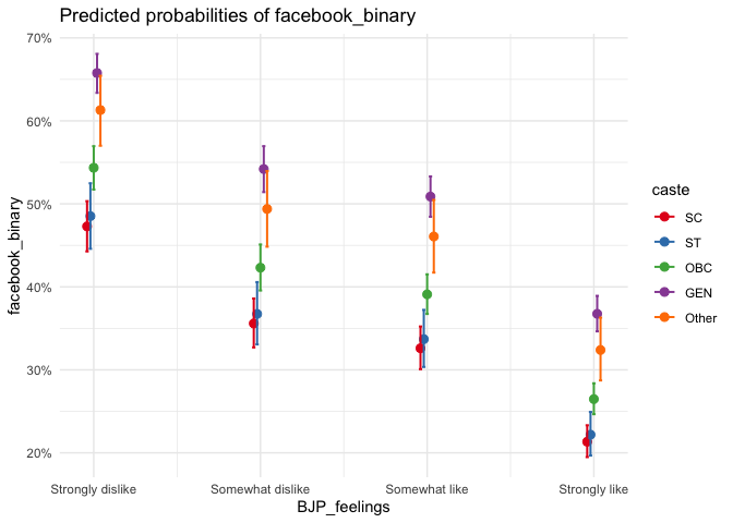
However, across caste lines, there are interesting patterns. We see that the general category who belong to the dominant castes are inclined to believe that facebook news is accurate, compared to the Scheduled Caste who are in the lowest of the caste hierarchy. Let me make a predicted probability graph to visualise it better.
plot_model(model_facebook, type = "pred",
     terms = c("BJP_feelings","caste")) +
  theme_minimal()
plot_model(model_facebook, type = "pred",
     terms = c("INC_feelings","caste")) +
  theme_minimal()
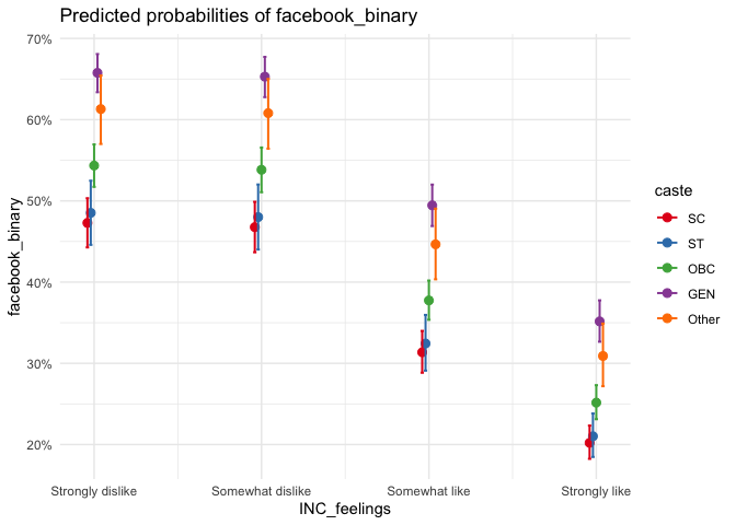
As we can see, the perception about Facebook is also stratified across caste-lines, in the same hierarchy. The dominant GEN believes facebook news to be more accurate, followed by the Other comprising of dominant castes, followed by OBC comprising of middle to backward castes, and followed closely by ST and SC who are in the bottom of the caste hierarchy.
Regression Model 2 - Whatsapp Accuracy:
In this second model, I will keep whatsapp\_binary as the dependent variable and logit regress it against BJP\_feelings, INC\_feelings, caste and political\_interest:
model_whatsapp <- glm(whatsapp_binary ~ BJP_feelings + INC_feelings + caste + political_interest,
              data = data, family = binomial(link="logit"))
tab_model(model_whatsapp, show.se = T, show.aic = T, show.loglik = T, transform = NULL)
| whatsapp\_binary | ||||
|---|---|---|---|---|
| Predictors | Log-Odds | std. Error | CI | p |
| (Intercept) | 0.14 | 0.06 | 0.02 – 0.26 | 0.024 |
| BJP\_feelings \[Somewhat dislike\] | -0.25 | 0.04 | -0.34 – -0.16 | <0.001 |
| BJP\_feelings \[Somewhat like\] | -0.60 | 0.03 | -0.67 – -0.54 | <0.001 |
| BJP\_feelings \[Strongly like\] | -1.34 | 0.03 | -1.41 – -1.27 | <0.001 |
| INC\_feelings \[Somewhat dislike\] | -0.26 | 0.03 | -0.32 – -0.20 | <0.001 |
| INC\_feelings \[Somewhat like\] | -0.75 | 0.03 | -0.80 – -0.69 | <0.001 |
| INC\_feelings \[Strongly like\] | -1.19 | 0.03 | -1.26 – -1.12 | <0.001 |
| caste \[ST\] | 0.19 | 0.07 | 0.05 – 0.34 | 0.008 |
| caste \[OBC\] | 0.26 | 0.04 | 0.17 – 0.34 | <0.001 |
| caste \[GEN\] | 0.84 | 0.04 | 0.77 – 0.93 | <0.001 |
| caste \[Other\] | 0.18 | 0.09 | 0.01 – 0.34 | 0.040 |
| political\_interest \[Not very interested\] | 0.61 | 0.06 | 0.49 – 0.74 | <0.001 |
| political\_interest \[Somewhat interested\] | 0.26 | 0.05 | 0.17 – 0.35 | <0.001 |
| political\_interest \[Very interested\] | 0.19 | 0.05 | 0.10 – 0.28 | <0.001 |
| political\_interest \[Extremely interested\] | -0.09 | 0.05 | -0.19 – 0.00 | 0.050 |
| Observations | 45792 | |||
| R2 Tjur | 0.104 | |||
| AIC | 55749.060 | |||
| log-Likelihood | -27859.530 | |||
In this model as well, we get a very weak association owing to the low R-square value, but we have a high AIC value and statistical signifance across many variables. Similar to the accuracy of facebook, people show a similar attitude towards whatsapp, as they might be treating it both under social media, attributing common characteristics. In this table also, we can see that no matter the feelings about either BJP or INC, people are less inclined to believe that whatsapp news is accurate. But as usual, I am more interested in how caste distrinution is present in this model, as we are seeing that the “Other” caste group is not showing a significat log-odds as it showed in the previous model. Let me create a predicted probability graph to visualise:
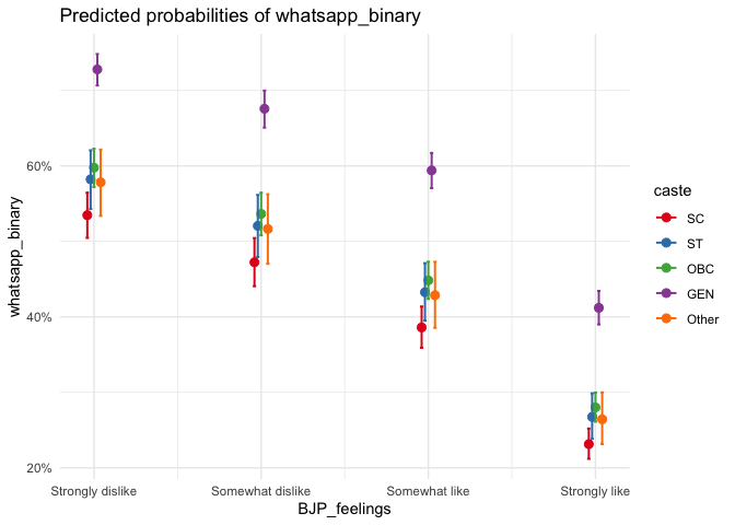
plot_model(model_whatsapp, type = "pred",
     terms = c("BJP_feelings","caste")) +
  theme_minimal()
plot_model(model_whatsapp, type = "pred",
     terms = c("INC_feelings","caste")) +
  theme_minimal()
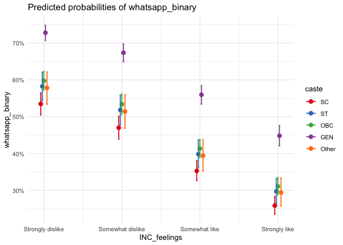
Here too, except the “Other” category, the line-up follows closely the caste hierarchy, but the dominant General category believes whatsapp news to be accurate more evidently here. This might probably have to do with their digital literacy and smartphone affordability, but this graph indicates the high mobility that the dominant castes enjoy in the digital space. One way to interpret is that the more we spend time on a social media, the more we tend to believe it as true, and this may indicate the higher trust of whatsapp news by the dominant general category. However, to see what news they are really consuming require a separate experiment with qualitative features.
DIAGNOSTICS
Since I am not directly comparing two models, I am not running a Likelihood Ratio Test or ROC curves. However, I shall run the Wald’s test to evaluate the statisitical significance individual coefficients in both the models. First in the Facebook model:
regTermTest(model_facebook, "BJP_feelings")

## Wald test for BJP_feelings
##  in glm(formula = facebook_binary ~ BJP_feelings + INC_feelings +
##     caste + political_interest, family = binomial(link = "logit"),
##     data = data)
## F =  476.8545  on  3  and  46545  df: p= < 2.22e-16

regTermTest(model_facebook, "INC_feelings")

## Wald test for INC_feelings
##  in glm(formula = facebook_binary ~ BJP_feelings + INC_feelings +
##     caste + political_interest, family = binomial(link = "logit"),
##     data = data)
## F =  577.5673  on  3  and  46545  df: p= < 2.22e-16

regTermTest(model_facebook, "caste")

## Wald test for caste
##  in glm(formula = facebook_binary ~ BJP_feelings + INC_feelings +
##     caste + political_interest, family = binomial(link = "logit"),
##     data = data)
## F =  175.0703  on  4  and  46545  df: p= < 2.22e-16

regTermTest(model_facebook, "political_interest")

## Wald test for political_interest
##  in glm(formula = facebook_binary ~ BJP_feelings + INC_feelings +
##     caste + political_interest, family = binomial(link = "logit"),
##     data = data)
## F =  58.29105  on  4  and  46545  df: p= < 2.22e-16
We see that all the p-values are low, indicating statistical significance of individual coeffecients. Let me take the test for Whatsapp model as well:
regTermTest(model_whatsapp, "BJP_feelings")

## Wald test for BJP_feelings
##  in glm(formula = whatsapp_binary ~ BJP_feelings + INC_feelings +
##     caste + political_interest, family = binomial(link = "logit"),
##     data = data)
## F =  693.6791  on  3  and  45777  df: p= < 2.22e-16

regTermTest(model_whatsapp, "INC_feelings")

## Wald test for INC_feelings
##  in glm(formula = whatsapp_binary ~ BJP_feelings + INC_feelings +
##     caste + political_interest, family = binomial(link = "logit"),
##     data = data)
## F =  500.8289  on  3  and  45777  df: p= < 2.22e-16

regTermTest(model_whatsapp, "caste")

## Wald test for caste
##  in glm(formula = whatsapp_binary ~ BJP_feelings + INC_feelings +
##     caste + political_interest, family = binomial(link = "logit"),
##     data = data)
## F =  241.0764  on  4  and  45777  df: p= < 2.22e-16

regTermTest(model_whatsapp, "political_interest")

## Wald test for political_interest
##  in glm(formula = whatsapp_binary ~ BJP_feelings + INC_feelings +
##     caste + political_interest, family = binomial(link = "logit"),
##     data = data)
## F =  74.91164  on  4  and  45777  df: p= < 2.22e-16
Again, we get low p-values, indicating statistical significance of individual coeffecients in this model as well.
CONCLUSION
Given the low value of R-square, I am unable to substantiate any association between people’s political preference or caste to their opinion about social media news, however, I was able to pinpoint a pattern of trust cutting across caste-lines rather than party-lines towards the social media news. This makes me think about the missing variables in this dataset such as the ability to buy a smartphone, digital literacy, etc. I consciously avoided education as a variable in my regression for theoretical reasons, since I intuitively do not give much value to the notion that school education in India could improve one’s perception about news accuracy. I believe that keeping these dependent variables and introducing new independentent variables in future models could shed light on how people’s motivated reasoning could affect their perception about social media news accuracy.
Co-Director
Global Governance Centre
Professor
International Relations and Political Science
President
Global Governance Research Centre Consortium
International institutions and political networks.