Henrique Sposito
- 1. Introduction
- 2. Data and Methodology
- 3. Data visualization
- 4. Regression models
- 5. Discussions and Conclusion
- References:
1. Introduction
Rooduijn and Burgoon (2018), in the article “The Paradox of Wellbeing: Do Unfavorable Socioeconomic and Sociocultural Contexts Deepen or Dampen Radical Left and Right Voting Among the Less Well-Off?”, find some interesting patterns related to when voters are more likely to choose radical left-wing and right-wing parties. The authors argue that “less well-off citizens might only vote for a radical party under more favorable circumstances - if, in other words, these circumstances are relatively ‘safe’ for radical experimentation” (Rooduijn and Burgoon 2018, p. 1746). However, the authors’ proposed mechanisms explaining experimentalism at the micro level remains underdeveloped theoretically. While experimentalism may indeed spur from perceptions of economic “safety” at the macro level, micro level dynamics for why voters conceive the possibility of voting for either left or right leaning radical parties are not given enough attention. The authors assume the less well-off are the voting base for all radical parties and, as such, they treat low income as their main independent variable, rather than income as a control variable. Although there are reasonable theoretical reasons that connect radical party voting to unemployment or poor economic conditions, there are also mix evidence on the relationship between income and voting for either, right-wing (see Rydgren and Ruth 2013) or left-wing (see Visser et al. 2014), radical parties in Europe. Moreover, the radical party’s literature illustrates that there are mixed socioeconomic and cultural correlations underlying radical party voting, and these are often country specific (see Rydgren and Ruth 2013).
Still, Rooduijn and Burgoon’s (2018) “safe experimentalism” claim appears reasonable and, if the authors are right, a condition under which radical party voting increases generally across European societies. Yet, the authors do not really test the “safe experimentalism” finding. Rooduijn and Burgoon operationalize economic growth as gross domestic product (GDP) per capita (among other things), which does not tell us much about when it is safe to experiment, but simply points to a relationship between macro-economics and radical party voting that could be explained in other ways than ‘experimentalism’. Nevertheless, the authors model right and left-wing voting in separate binary regressions but argue that the experimentalist finding holds for right and left-wing voting without testing them altogether. The claim is even more contentious taking into consideration the fact that radical parties are not evenly distributed across societies. This is evident in the dataset as many of the coded countries have either only right-wing radical parties (Austria and Belgium for example), or only left-wing radical parties (Czech Republic and Ireland for example).
There are two reasons to attempt to verify and expand Rooduijn and Burgoon’s (2018) apparent findings. First, if “safe experimentalism” holds, then a more specific model for when radical parties become more appealing to voters can be developed. This, in turn, could be an important general finding. Second, the election of radical parties over mainstream parties at the national level is a relatively rare event with low rates of occurrence over time for a variety of reasons (e.g. campaign budgets and/or incumbent’s advantage). In such, binary regressions or linear models may not account well for the time or country specific effect variation within the data, as Beck et al. (1998) and Wooldridge (2012) have argued elsewhere. Rather, a panel data model may be more appropriate to analyze the topic and datasets.
Likewise, radical left-wing and right-wing parties are often closer to each other in relation policy preferences (e.g. protectionism and authoritarianism), than they are to mainstream parties’ policy preferences (see Taylor 2006). For this theoretical reason, treating radical left-wing and right-wing parties across countries in separate regression models may be fallacious, as they often reflect similar policy preferences and appeal to rather similar demographics in countries where one or the other are absent. This theoretical understanding of party politics and ideology alongside the reasonable “safe experimentalism” claim allows me to hypothesize that: The likelihood of voting for radical parties in Europe increases when macroeconomic conditions are minimally stable and trust in politics and is low. In this sense, radical party voting increases with dissatisfaction with politics only when economic conditions are stable enough for experimenting politically. Nevertheless, three considerations must be made regarding the hypothesis above. First, because the main claim of this paper is taken from Rooduijn and Burgoon’s (2018) article, a modified version of their dataset is used. Since the dataset contains data only on some European countries, the hypothesis is restricted to Europe. Second, because the predictor variables hypothesized (minimally stable macroeconomic conditions and political trust) may depend on each other, it is expected that there will be some degree of multicollinearity amongst predictors. Finally, there are several reasons why individuals vote for radical, left or right-wing, parties and these are not always correlated with economic conditions or political trust (see Rydgren and Ruth 2013; Visser et al. 2014). Yet, if economic conditions and political trust delineate underlying conditions that correlate to increases in radical voting, this could be an important correlational finding. This paper does not attempt to replicate Rooduijn and Burgoon’s (2018) findings, rather it attempts to corroborate if their claim regarding “safe experimentalism” holds once the dataset is modified and different regression approaches are attempted.
2. Data and Methodology
Rooduijn and Burgoon’s (2018) dataset, made available in the article’s replication materials, is adapted and modified to test the hypothesis above. The dataset contains individual level data for the twenty-one European countries who participated in seven waves of the European Social Survey (ESS) that took place from 2002 to 2014. The individual level data were aggregated by variables’ average for a respective country-year. This is done because, contrary to Rooduijn and Burgoon’s (2018), I am are interested in the variation in radical party voting by country-year rather than subgroups of the population. Nevertheless, the main dependent variables coded by the authors’, radical left and right-wing voting over mainstream left or right leaning parties, was missing around 25% of the values. This is most likely due to individual respondents, who declared to have voted for a political party which was not identified by the authors or participants who refused to answer the question during the ESS survey round. Following what Rooduijn and Burgoon’s (2018) did as a robustness check of their findings (see online appendixes), all the missing values were changed to zeros before these two variables were averaged. This means all missing values were coded as if they had not voted for a radical party. Such decreases the likelihood of finding statistically significant results, but also increases the robustness of any possible findings using the data. The main dependent variable here, radical party voting, was recoded as the sum of radical left-wing and right-wing party voting for the specific country-year. Beyond missing values for the dependent variables, the dataset also contained several countries that did not participate in all the waves of the ESS taking place from 2002 to 2014. Hence, for some countries there are more country-year observations than others, although most countries in the dataset participated in at least five out of the seven waves during the time period.
As for the main predictor variables, the average values for political trust (poltrst) and trust in politicians (trstplt) for a respective country-year, already present in the dataset, are how political trust was operationalized. Minimally stable economic conditions that allow for experimentalism was operationalized using the Global Economic Indicators data variable for GDP growth per country-year (available in the World Bank database). For each round of the ESS, the data relative to a respective country’s GDP growth for the year prior was added to the dataset (because the ESS often takes place during the summer months). However, since the “safe experimentalism” hypothesis holds that safe enough conditions for experimentalism correlate with radical voting, GDP growth per se cannot be used. If the hypothesis holds, voting for radical parties would decrease in times of economic boom or times of economic recession because these are “unsafe” times for experimentalism. Thus, a categorical variable for economic growth by country-year was created. The categorical variable for GDP growth (gdpcat) has seven categories. The categories are: “minstable” (for GDP growth/decrease ranging from - 1% to 1% for the previous year), “normalgrowth” (1.01% to 3%), “exceptg” (3.01% to 5%), “boom” (> 5% ), “downturn” (-1.01% to -3%), “shrink” (-3.01% to -5%) and “recession” (< -5%). Additionally, because I hypothesize about both political trust and economic conditions joint effects on radical voting, a dummy variable for “safe experimentalism” (safexp) was created. The dummy variable has the score of 1 if, for a respective country-year, political trust levels are below the country’s average and economic growth falls into “minstable”, “normalgrowth” or “downturn” categories. The dummy variable is coded 0 otherwise.
The different underlying approaches to estimate relationships and effects used are pooled OLS, fixed-effect and random effects-models. Although it is unlikely that pooled OLS models are appropriate to analyze this data (see Wooldridge 2012), the sample contains countries which did not participated in all of the ESS waves considered and, for that reason, there is a small possibility that there are no significant random or individual time effects. Likely, because this is a panel dataset, fixed or random-effects approaches are more suited. Since the pertinent dependent and independent variables, as radical voting or political trust, may have relatively little variation across unit and time, there is reason to believe a random-effects model would fit the data better. At the same time, countries may share distinctive attributes that correlate with regressors, which could indicate that the fixed-effects model would produce superior estimates. For these reasons, the three approaches are modeled while post-estimation tests are used to determine model fit.
In total six regression models are run using the PLM package dedicated to panel data estimations. The first three models contain the same four predictor variables (trstplt, poltrst, gdpcat and safexp) and are run as pooled OLS, fixed-effects and random-effects. The following three models are the same as above, but several control variables are added. The control variables added are average income of participants for each country/year (income), average education of participants by country/year (educ), average rate of participants who were unemployed (unemp), average age of participants by country/year (age), average rate of urban to rural respondents (ruralurban), percent GDP growth for previous year (gdpgrow), average immigrant attitudes for country/year (imbgeco) - as a control for right wing radical party voting - and views about inequality (incdif) - as a control for left wing radical party voting. The table below summarizes the modified dataset and illustrate some of the inconsistencies with the data mentioned above, as missing country data for some years.
3. Data visualization
library(readxl)

df <- read_excel("d4.xlsx")

dfinal <- as.data.frame(df)

table1::table1(~.,data=dfinal, topclass="Rtable1-zebra")

## [1] "<table class=\"Rtable1-zebra\">\n<thead>\n<tr>\n<th class='rowlabel firstrow lastrow'></th>\n<th class='firstrow lastrow'><span class='stratlabel'>Overall<br><span class='stratn'>(N=130)</span></span></th>\n</tr>\n</thead>\n<tbody>\n<tr>\n<td class='rowlabel firstrow'><span class='varlabel'>country</span></td>\n<td class='firstrow'></td>\n</tr>\n<tr>\n<td class='rowlabel'>Austria</td>\n<td>4 (3.1%)</td>\n</tr>\n<tr>\n<td class='rowlabel'>Belgium</td>\n<td>7 (5.4%)</td>\n</tr>\n<tr>\n<td class='rowlabel'>Czech Republic</td>\n<td>6 (4.6%)</td>\n</tr>\n<tr>\n<td class='rowlabel'>Denmark</td>\n<td>7 (5.4%)</td>\n</tr>\n<tr>\n<td class='rowlabel'>Finland</td>\n<td>7 (5.4%)</td>\n</tr>\n<tr>\n<td class='rowlabel'>France</td>\n<td>7 (5.4%)</td>\n</tr>\n<tr>\n<td class='rowlabel'>Germany</td>\n<td>7 (5.4%)</td>\n</tr>\n<tr>\n<td class='rowlabel'>Great Britain</td>\n<td>6 (4.6%)</td>\n</tr>\n<tr>\n<td class='rowlabel'>Greece</td>\n<td>4 (3.1%)</td>\n</tr>\n<tr>\n<td class='rowlabel'>Hungary</td>\n<td>6 (4.6%)</td>\n</tr>\n<tr>\n<td class='rowlabel'>Ireland</td>\n<td>7 (5.4%)</td>\n</tr>\n<tr>\n<td class='rowlabel'>Italy</td>\n<td>3 (2.3%)</td>\n</tr>\n<tr>\n<td class='rowlabel'>Netherlands</td>\n<td>7 (5.4%)</td>\n</tr>\n<tr>\n<td class='rowlabel'>Norway</td>\n<td>7 (5.4%)</td>\n</tr>\n<tr>\n<td class='rowlabel'>Poland</td>\n<td>7 (5.4%)</td>\n</tr>\n<tr>\n<td class='rowlabel'>Portugal</td>\n<td>6 (4.6%)</td>\n</tr>\n<tr>\n<td class='rowlabel'>Slovakia</td>\n<td>5 (3.8%)</td>\n</tr>\n<tr>\n<td class='rowlabel'>Slovenia</td>\n<td>7 (5.4%)</td>\n</tr>\n<tr>\n<td class='rowlabel'>Spain</td>\n<td>6 (4.6%)</td>\n</tr>\n<tr>\n<td class='rowlabel'>Sweden</td>\n<td>7 (5.4%)</td>\n</tr>\n<tr>\n<td class='rowlabel lastrow'>Switzerland</td>\n<td class='lastrow'>7 (5.4%)</td>\n</tr>\n<tr>\n<td class='rowlabel firstrow'><span class='varlabel'>year</span></td>\n<td class='firstrow'></td>\n</tr>\n<tr>\n<td class='rowlabel'>Mean (SD)</td>\n<td>2010 (3.94)</td>\n</tr>\n<tr>\n<td class='rowlabel lastrow'>Median [Min, Max]</td>\n<td class='lastrow'>2010 [2000, 2010]</td>\n</tr>\n<tr>\n<td class='rowlabel firstrow'><span class='varlabel'>trstplt</span></td>\n<td class='firstrow'></td>\n</tr>\n<tr>\n<td class='rowlabel'>Mean (SD)</td>\n<td>3.68 (1.03)</td>\n</tr>\n<tr>\n<td class='rowlabel lastrow'>Median [Min, Max]</td>\n<td class='lastrow'>3.51 [1.36, 5.61]</td>\n</tr>\n<tr>\n<td class='rowlabel firstrow'><span class='varlabel'>poltrst</span></td>\n<td class='firstrow'></td>\n</tr>\n<tr>\n<td class='rowlabel'>Mean (SD)</td>\n<td>4.13 (1.04)</td>\n</tr>\n<tr>\n<td class='rowlabel lastrow'>Median [Min, Max]</td>\n<td class='lastrow'>4.08 [1.70, 6.06]</td>\n</tr>\n<tr>\n<td class='rowlabel firstrow'><span class='varlabel'>incdif</span></td>\n<td class='firstrow'></td>\n</tr>\n<tr>\n<td class='rowlabel'>Mean (SD)</td>\n<td>3.82 (0.330)</td>\n</tr>\n<tr>\n<td class='rowlabel lastrow'>Median [Min, Max]</td>\n<td class='lastrow'>3.82 [2.96, 4.43]</td>\n</tr>\n<tr>\n<td class='rowlabel firstrow'><span class='varlabel'>unemp</span></td>\n<td class='firstrow'></td>\n</tr>\n<tr>\n<td class='rowlabel'>Mean (SD)</td>\n<td>0.0486 (0.0257)</td>\n</tr>\n<tr>\n<td class='rowlabel lastrow'>Median [Min, Max]</td>\n<td class='lastrow'>0.0456 [0.00882, 0.151]</td>\n</tr>\n<tr>\n<td class='rowlabel firstrow'><span class='varlabel'>educ</span></td>\n<td class='firstrow'></td>\n</tr>\n<tr>\n<td class='rowlabel'>Mean (SD)</td>\n<td>3.07 (0.383)</td>\n</tr>\n<tr>\n<td class='rowlabel lastrow'>Median [Min, Max]</td>\n<td class='lastrow'>3.09 [1.86, 3.69]</td>\n</tr>\n<tr>\n<td class='rowlabel firstrow'><span class='varlabel'>ruralurban</span></td>\n<td class='firstrow'></td>\n</tr>\n<tr>\n<td class='rowlabel'>Mean (SD)</td>\n<td>1.61 (0.0993)</td>\n</tr>\n<tr>\n<td class='rowlabel lastrow'>Median [Min, Max]</td>\n<td class='lastrow'>1.61 [1.40, 1.80]</td>\n</tr>\n<tr>\n<td class='rowlabel firstrow'><span class='varlabel'>age</span></td>\n<td class='firstrow'></td>\n</tr>\n<tr>\n<td class='rowlabel'>Mean (SD)</td>\n<td>48.8 (1.97)</td>\n</tr>\n<tr>\n<td class='rowlabel lastrow'>Median [Min, Max]</td>\n<td class='lastrow'>48.6 [43.8, 54.8]</td>\n</tr>\n<tr>\n<td class='rowlabel firstrow'><span class='varlabel'>imbgeco</span></td>\n<td class='firstrow'></td>\n</tr>\n<tr>\n<td class='rowlabel'>Mean (SD)</td>\n<td>5.10 (0.654)</td>\n</tr>\n<tr>\n<td class='rowlabel lastrow'>Median [Min, Max]</td>\n<td class='lastrow'>5.09 [3.79, 6.90]</td>\n</tr>\n<tr>\n<td class='rowlabel firstrow'><span class='varlabel'>income</span></td>\n<td class='firstrow'></td>\n</tr>\n<tr>\n<td class='rowlabel'>Mean (SD)</td>\n<td>5.68 (1.22)</td>\n</tr>\n<tr>\n<td class='rowlabel'>Median [Min, Max]</td>\n<td>5.73 [3.14, 8.46]</td>\n</tr>\n<tr>\n<td class='rowlabel lastrow'>Missing</td>\n<td class='lastrow'>6 (4.6%)</td>\n</tr>\n<tr>\n<td class='rowlabel firstrow'><span class='varlabel'>stfeco</span></td>\n<td class='firstrow'></td>\n</tr>\n<tr>\n<td class='rowlabel'>Mean (SD)</td>\n<td>4.62 (1.47)</td>\n</tr>\n<tr>\n<td class='rowlabel lastrow'>Median [Min, Max]</td>\n<td class='lastrow'>4.73 [1.34, 7.98]</td>\n</tr>\n<tr>\n<td class='rowlabel firstrow'><span class='varlabel'>radicalvote</span></td>\n<td class='firstrow'></td>\n</tr>\n<tr>\n<td class='rowlabel'>Mean (SD)</td>\n<td>0.0694 (0.0573)</td>\n</tr>\n<tr>\n<td class='rowlabel lastrow'>Median [Min, Max]</td>\n<td class='lastrow'>0.0586 [0, 0.228]</td>\n</tr>\n<tr>\n<td class='rowlabel firstrow'><span class='varlabel'>gdpgrow</span></td>\n<td class='firstrow'></td>\n</tr>\n<tr>\n<td class='rowlabel'>Mean (SD)</td>\n<td>1.40 (3.05)</td>\n</tr>\n<tr>\n<td class='rowlabel lastrow'>Median [Min, Max]</td>\n<td class='lastrow'>1.80 [-8.07, 10.8]</td>\n</tr>\n<tr>\n<td class='rowlabel firstrow'><span class='varlabel'>gdpcat</span></td>\n<td class='firstrow'></td>\n</tr>\n<tr>\n<td class='rowlabel'>boom</td>\n<td>12 (9.2%)</td>\n</tr>\n<tr>\n<td class='rowlabel'>downturn</td>\n<td>6 (4.6%)</td>\n</tr>\n<tr>\n<td class='rowlabel'>exceptg</td>\n<td>23 (17.7%)</td>\n</tr>\n<tr>\n<td class='rowlabel'>minstable</td>\n<td>27 (20.8%)</td>\n</tr>\n<tr>\n<td class='rowlabel'>normalgrowth</td>\n<td>48 (36.9%)</td>\n</tr>\n<tr>\n<td class='rowlabel'>recession</td>\n<td>6 (4.6%)</td>\n</tr>\n<tr>\n<td class='rowlabel lastrow'>shrink</td>\n<td class='lastrow'>8 (6.2%)</td>\n</tr>\n<tr>\n<td class='rowlabel firstrow'><span class='varlabel'>safexp</span></td>\n<td class='firstrow'></td>\n</tr>\n<tr>\n<td class='rowlabel'>Mean (SD)</td>\n<td>0.300 (0.460)</td>\n</tr>\n<tr>\n<td class='rowlabel lastrow'>Median [Min, Max]</td>\n<td class='lastrow'>0 [0, 1.00]</td>\n</tr>\n</tbody>\n</table>\n"
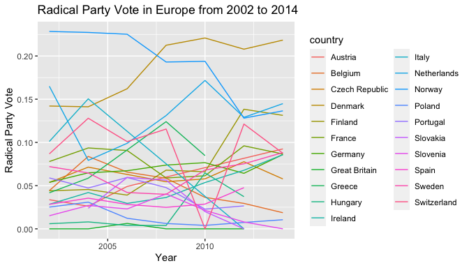
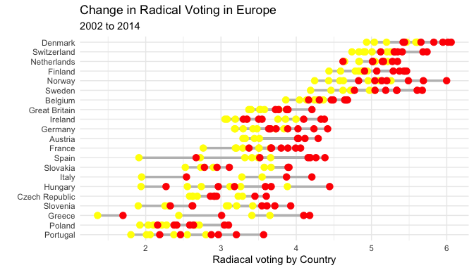
The figure below illustrates the dependent variable, radical party voting, across European countries during the period.
Radical Party Voting in Europe from 2002 to 2014
library(tidyverse)

## ── Attaching packages ───────────────────────────────────────────────── tidyverse 1.3.0 ──

## ✓ ggplot2 3.3.0     ✓ purrr   0.3.4
## ✓ tibble  3.0.1     ✓ dplyr   0.8.5
## ✓ tidyr   1.1.0     ✓ stringr 1.4.0
## ✓ readr   1.3.1     ✓ forcats 0.5.0

## ── Conflicts ──────────────────────────────────────────────────── tidyverse_conflicts() ──
## x dplyr::filter() masks stats::filter()
## x dplyr::lag()    masks stats::lag()

library(ggplot2)

ggplot(dfinal, mapping = aes(x = year, y = radicalvote)) + geom_line(aes(color = country)) +
  labs(title="Radical Party Vote in Europe from 2002 to 2014", x = "Year", y = "Radical Party Vote")
library(ggalt)

## Registered S3 methods overwritten by 'ggalt':
##   method                  from
##   grid.draw.absoluteGrob  ggplot2
##   grobHeight.absoluteGrob ggplot2
##   grobWidth.absoluteGrob  ggplot2
##   grobX.absoluteGrob      ggplot2
##   grobY.absoluteGrob      ggplot2

plotdata_wide <- spread(dfinal, year, radicalvote)

names(plotdata_wide) <- c("country", "y2002", "y2014")

ggplot(plotdata_wide,
       aes(y = reorder(country, y2002),
           x = y2002,
           xend = y2014)) +
  geom_dumbbell(size = 1.2,
                size_x = 3,
                size_xend = 3,
                colour = "grey",
                colour_x = "yellow",
                colour_xend = "red") +
  theme_minimal() +
  labs(title = "Change in Radical Voting in Europe",
       subtitle = "2002 to 2014",
       x = "Radiacal voting by Country",
       y = "") + theme_minimal()
library(CGPfunctions)

## Registered S3 methods overwritten by 'lme4':
##   method                          from
##   cooks.distance.influence.merMod car
##   influence.merMod                car
##   dfbeta.influence.merMod         car
##   dfbetas.influence.merMod        car

slope <- dfinal %>% filter(year %in% c(2002, 2008, 2014)) %>% mutate(year = factor(year))

newggslopegraph(slope, year, radicalvote, country, DataTextSize = 3) +labs(title="Change in Radical voting by Country in Europe from 2002 to 2014")

##
## Converting 'year' to an ordered factor
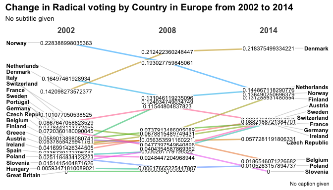
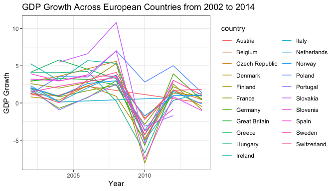
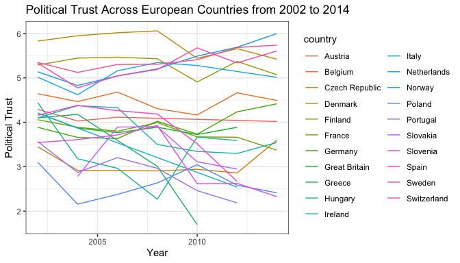
Note that radical party voting has increased in most countries surveyed from 2002 to 2014, although this increase appears to be modest. Moreover, plotting GDP growth (gdpgrow - non categorical) across these European countries shows that GDP growth and downturns appear to happen simultaneously for most countries, though the dimensions differ (see below). This is expected since all the countries belong to the same geographical region. While political trust does not appear to vary much within countries during the period, levels appear to fluctuate farther across countries (see below).
3.1 Visualization the independent variable and their correlations
ggplot(dfinal, mapping = aes(x = year, y = gdpgrow)) + geom_line(aes(color = country)) + labs(title = "GDP Growth Across European Countries from 2002 to 2014",
       x = "Year",
       y = "GDP Growth")
ggplot(dfinal, mapping = aes(x = year, y = poltrst)) + geom_line(aes(color = country)) + labs(title = "Political Trust Across European Countries from 2002 to 2014",
       x = "Year",
       y = "Political Trust")
Though it was expected that the political trust and economic growth variables would correlate, this appears not to be the case. The graph below shows that their relationship is not linear, and the correlation test (cor.test) confirms that their correlation is minimal.
3.2 Visualizing the Relationships between Independent Variables
ggplot(dfinal, mapping = aes(x = poltrst, y = gdpgrow)) + geom_line(aes(color = country)) + labs(title = "Correlations Between GDP Growth and Political Trust Across European Countries from 2002 to 2014",
       x = "Political Trust",
       y = "GDP Growth")
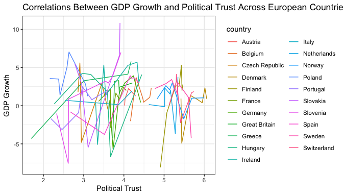
cor.test(dfinal$poltrst, dfinal$gdpgrow)

##
##  Pearson's product-moment correlation
##
## data:  dfinal$poltrst and dfinal$gdpgrow
## t = 0.47918, df = 128, p-value = 0.6326
## alternative hypothesis: true correlation is not equal to 0
## 95 percent confidence interval:
##  -0.1308235  0.2129503
## sample estimates:
##        cor
## 0.04231575
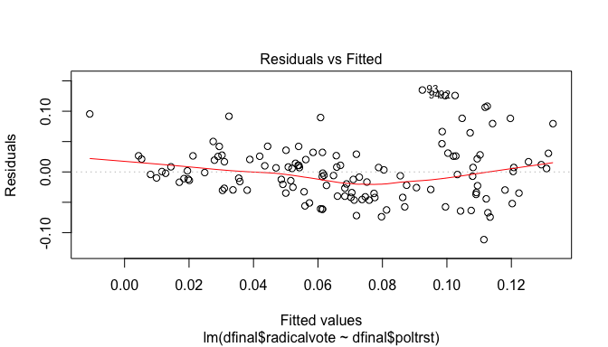
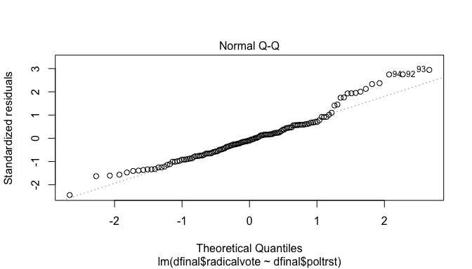
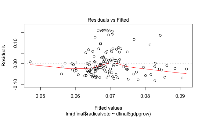
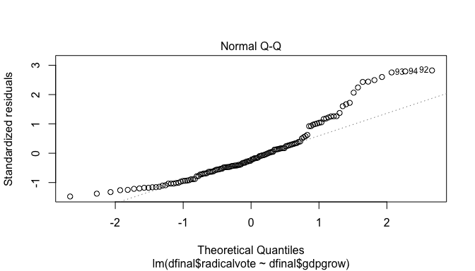
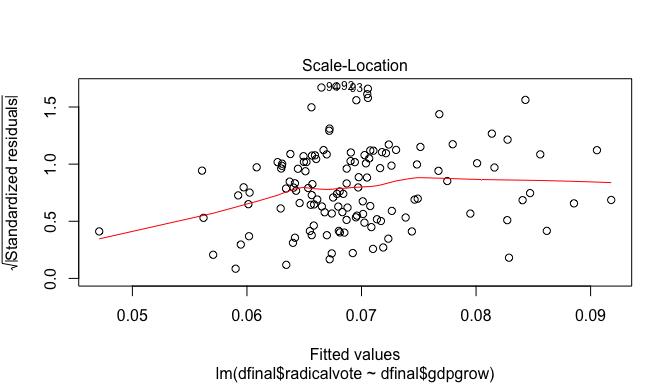
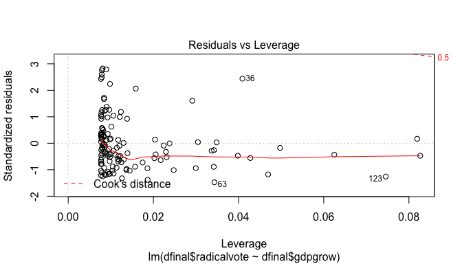
Finally, a simple linear plot of the correlations between radical voting and political trust, as well as radical voting and GDP growth (below), illustrates no visible linear relationship between the variables.
3.3 Plotting Relationships between Independent Variables and Dependent Variable
plot(lm(dfinal$radicalvote ~ dfinal$poltrst))
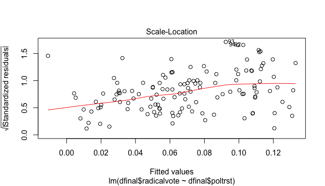
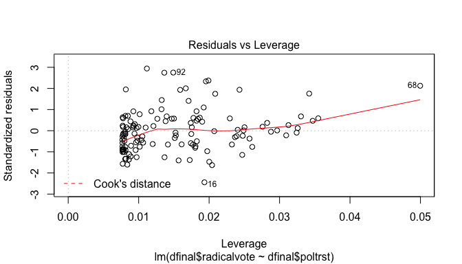
plot(lm(dfinal$radicalvote ~ dfinal$gdpgrow))
4.Regression models
The table below shows the results of the 6 regression models. The three first models are run without any control variables, while the 3 last contain several control variables.
library(plm)

##
## Attaching package: 'plm'

## The following objects are masked from 'package:dplyr':
##
##     between, lag, lead

pols1 <- plm(radicalvote ~ trstplt + poltrst + as.factor(gdpcat) + as.factor(safexp), data=dfinal, model = "pooling", index = c("country", "year"))

fe1 <- plm(radicalvote ~ trstplt + poltrst + as.factor(gdpcat) + as.factor(safexp), data=dfinal, model = "within", index = c("country", "year"))

re1 <- plm(radicalvote ~ trstplt + poltrst + as.factor(gdpcat) + as.factor(safexp) , data=dfinal, model = "random", index = c("country", "year"))

pols2 <- plm(radicalvote ~ trstplt + poltrst + as.factor(gdpcat) + as.factor(safexp) + income + unemp + educ + age + ruralurban + imbgeco + incdif + gdpgrow + stfeco, data=dfinal, model = "pooling", index = c("country", "year"))

fe2 <- plm(radicalvote ~ trstplt + poltrst + as.factor(gdpcat) + as.factor(safexp) + income + unemp + educ + age + ruralurban + imbgeco + incdif + gdpgrow + stfeco, data=dfinal, model = "within", index = c("country", "year"))

re2 <- plm(radicalvote ~ trstplt + poltrst + as.factor(gdpcat) + as.factor(safexp) + income + unemp + educ + age + ruralurban + imbgeco + incdif + gdpgrow + stfeco, data=dfinal, model = "random", index = c("country", "year"))

library(stargazer)

##
## Please cite as:

##  Hlavac, Marek (2018). stargazer: Well-Formatted Regression and Summary Statistics Tables.

##  R package version 5.2.2. https://CRAN.R-project.org/package=stargazer

stargazer(pols1, fe1, re1, type="text", title = "Regression Results for Models without Control Variables", column.labels = c("Pooled OLS", "Fixed-Effects", "Random-Effects") ,dep.var.labels=c("Radical Party Voting in Europe"), align=TRUE)

##
## Regression Results for Models without Control Variables
## ========================================================================================
##                                                  Dependent variable:
##                               ----------------------------------------------------------
##                                             Radical Party Voting in Europe
##                                     Pooled OLS           Fixed-Effects    Random-Effects
##                                         (1)                   (2)              (3)
## ----------------------------------------------------------------------------------------
## trstplt                                0.022                 0.015            0.029
##                                       (0.023)               (0.044)          (0.032)
##
## poltrst                                0.012                -0.007            -0.005
##                                       (0.023)               (0.041)          (0.031)
##
## as.factor(gdpcat)downturn             -0.007               -0.035**           -0.027
##                                       (0.024)               (0.018)          (0.018)
##
## as.factor(gdpcat)exceptg              -0.002                 0.004            0.007
##                                       (0.016)               (0.012)          (0.012)
##
## as.factor(gdpcat)minstable            0.029*                -0.003            0.007
##                                       (0.017)               (0.013)          (0.013)
##
## as.factor(gdpcat)normalgrowth          0.007                -0.0001           0.004
##                                       (0.015)               (0.011)          (0.011)
##
## as.factor(gdpcat)recession             0.015                 0.012            0.020
##                                       (0.022)               (0.015)          (0.015)
##
## as.factor(gdpcat)shrink               0.038*                 0.014            0.026*
##                                       (0.020)               (0.015)          (0.015)
##
## as.factor(safexp)1                    0.018*                 0.013           0.020**
##                                       (0.011)               (0.008)          (0.008)
##
## Constant                             -0.078***                                -0.028
##                                       (0.021)                                (0.028)
##
## ----------------------------------------------------------------------------------------
## Observations                            130                   130              130
## R2                                     0.453                 0.088            0.166
## Adjusted R2                            0.411                -0.176            0.104
## F Statistic                   11.020*** (df = 9; 120) 1.074 (df = 9; 100)   23.927***
## ========================================================================================
## Note:                                                        *p<0.1; **p<0.05; ***p<0.01

stargazer(pols2, fe2, re2, type="text", title = "Regression Results with Control Variables", column.labels = c("Pooled OLS", "Fixed-Effects", "Random-Effects") ,dep.var.labels=c("Radical Party Voting in Europe"), align=TRUE)

##
## Regression Results with Control Variables
## ========================================================================================
##                                                  Dependent variable:
##                               ----------------------------------------------------------
##                                             Radical Party Voting in Europe
##                                     Pooled OLS           Fixed-Effects    Random-Effects
##                                         (1)                   (2)              (3)
## ----------------------------------------------------------------------------------------
## trstplt                                0.011                 0.009            0.020
##                                       (0.034)               (0.050)          (0.035)
##
## poltrst                                0.024                0.0005            0.011
##                                       (0.032)               (0.047)          (0.034)
##
## as.factor(gdpcat)downturn              0.025                -0.052            -0.026
##                                       (0.058)               (0.039)          (0.043)
##
## as.factor(gdpcat)exceptg               0.009                -0.003            0.008
##                                       (0.024)               (0.016)          (0.018)
##
## as.factor(gdpcat)minstable             0.044                -0.020            0.002
##                                       (0.041)               (0.028)          (0.031)
##
## as.factor(gdpcat)normalgrowth          0.018                -0.010            0.0002
##                                       (0.030)               (0.020)          (0.022)
##
## as.factor(gdpcat)recession             0.057                -0.022            0.007
##                                       (0.086)               (0.058)          (0.065)
##
## as.factor(gdpcat)shrink                0.064                -0.006            0.019
##                                       (0.072)               (0.047)          (0.054)
##
## as.factor(safexp)1                     0.018                 0.007            0.017*
##                                       (0.012)               (0.009)          (0.009)
##
## income                                -0.003                 0.001            0.002
##                                       (0.005)               (0.003)          (0.004)
##
## unemp                                 -0.139                -0.064            0.076
##                                       (0.237)               (0.238)          (0.215)
##
## educ                                   0.021                 0.018            0.027*
##                                       (0.015)               (0.023)          (0.015)
##
## age                                   -0.002                 0.001           -0.0005
##                                       (0.003)               (0.002)          (0.002)
##
## ruralurban                            0.091*                0.219**          0.117**
##                                       (0.052)               (0.088)          (0.058)
##
## imbgeco                               -0.001                 0.007            -0.003
##                                       (0.010)               (0.014)          (0.011)
##
## incdif                                -0.008                 0.041            0.001
##                                       (0.023)               (0.031)          (0.022)
##
## gdpgrow                                0.003                -0.002            -0.001
##                                       (0.007)               (0.004)          (0.005)
##
## stfeco                                -0.004                -0.004            -0.005
##                                       (0.007)               (0.005)          (0.006)
##
## Constant                              -0.144                                  -0.280
##                                       (0.200)                                (0.194)
##
## ----------------------------------------------------------------------------------------
## Observations                            124                   124              124
## R2                                     0.489                 0.218            0.288
## Adjusted R2                            0.402                -0.132            0.165
## F Statistic                   5.593*** (df = 18; 105) 1.316 (df = 18; 85)   42.370***
## ========================================================================================
## Note:                                                        *p<0.1; **p<0.05; ***p<0.01

# I could not put all the models in the same table because the HTML file only shows4 models at a time when this is done. This is why the tables are split in two.
From the results tables, we do not see many statistically significant correlations between predictors and radical voting across the regression models. In the first pooled OLS model, the GDP growth categorical variables for minimally stable economic conditions (minstable) and economic shrink (shrink) are statistically significant (at the 0.1 P < 0.1 level) and appear to correlate with radical voting, in relation to the reference category (economic boom). As well, the safe experimentalism (safexp) dummy variable is statistically significant (at the P < 0.1 level). However, once several control variables are added to the same pooled OLS model, the only statistically significant predictor becomes the average rate of rural to urban (ruralurban) participants surveyed (at the 0.1 P-value level). Alternatively, in the first fixed-effects model only the GDP categorical variable for economic downturn (downturn) is statistically significant (at the 0.05 level). In the second fixed-effects model, with the control variables, downturn economic conditions (downturn) remains statistically significant alongside the average rate of rural to urban (ruralurban) participants (both at the P < 0.05 level). Nonetheless, in the first random-effects model, GDP growth categorical variables for economic shrink (shrink) is statistically significant (at the 0.1 P < 0.1 level), alongside the safe experimentalism (safexp) dummy variable (at the P < 0.5 level). In the second random-effects model, the safe experimentalism (safexp) dummy variable, the average education level of participants (educ) and the average rate of rural to urban (ruralurban) participants are statistically significant (all three at the P < 0.1 level). Yet, none of the models appears to be a good fit prima-facie or capture the variance in the dependent variable well, judging by adjusted R squared scores, coefficient values and standard errors. Moreover, the models do not appear to provide enough evidence that radical voting correlates consistently across in statistically significant ways with economically stable conditions or decreases in levels of political trust (or both).
4.1 Post-Estimation Tests
pbsytest(pols1)

##
##  Bera, Sosa-Escudero and Yoon locally robust test - unbalanced panel
##
## data:  formula
## chisq = 9.1758, df = 1, p-value = 0.002452
## alternative hypothesis: AR(1) errors sub random effects

pbsytest(pols2)

##
##  Bera, Sosa-Escudero and Yoon locally robust test - unbalanced panel
##
## data:  formula
## chisq = 11.484, df = 1, p-value = 0.000702
## alternative hypothesis: AR(1) errors sub random effects

plmtest(pols1)

##
##  Lagrange Multiplier Test - (Honda) for unbalanced panels
##
## data:  radicalvote ~ trstplt + poltrst + as.factor(gdpcat) + as.factor(safexp)
## normal = 9.4342, p-value < 2.2e-16
## alternative hypothesis: significant effects

plmtest(pols2)

##
##  Lagrange Multiplier Test - (Honda) for unbalanced panels
##
## data:  radicalvote ~ trstplt + poltrst + as.factor(gdpcat) + as.factor(safexp) +  ...
## normal = 8.7025, p-value < 2.2e-16
## alternative hypothesis: significant effects

phtest(fe1,re1)

##
##  Hausman Test
##
## data:  radicalvote ~ trstplt + poltrst + as.factor(gdpcat) + as.factor(safexp)
## chisq = 2.8326, df = 9, p-value = 0.9706
## alternative hypothesis: one model is inconsistent

phtest(fe2,re2)

##
##  Hausman Test
##
## data:  radicalvote ~ trstplt + poltrst + as.factor(gdpcat) + as.factor(safexp) +  ...
## chisq = 82.041, df = 18, p-value = 3.756e-10
## alternative hypothesis: one model is inconsistent
The Bera, Sosa-Escudero and Yoon locally robust test (pbsytest) performed on the pooled OLS regressions (above) allows us to reject the null hypothesis and confirm that errors are either serially correlated or randomly correlated; this means that the pooled OLS models are not appropriate to analyze the data. This is also confirmed by the Lagrange Multiplier Test (plmtest) which indicates that there are significant individual or time effects present on both pooled OLS models. When it comes to choosing between fixed or random-effects models, the Hausman test (phtest) allows us to can reject the null hypothesis that errors are not correlated to the independent variables. Thus, it indicates that the errors are indeed correlated with regressors and that there is no need to use random-effects; that both fixed-effects models are preferred over the random effects’ models. Given that we know that the pooled OLS models are not adequate for the data, and that neither the fixed-effects or random effects models give us many statistically significant results or appear to explain much of the variance in the dependent variable, there is no point in going further to check if the models violate other assumptions. Rather it is better to re-think the relationships theoretically, how to operationalize the variables hypothesized and try to find better datasets to test the hypothesis.
5. Discussions and Conclusion
Although none of the regression models above shows many (or consistent) statistically significant results, the “safe experimentalism” hypothesis remains a reasonable claim that should be further addressed in the future. This should be done with better data and better operationalizations of macro-economically safe conditions. While this paper did not attempt to replicate Rooduijn and Burgoon’s (2018), their claimed findings that: “individual hardship spurs radical left and right voting, this is the case mainly when aggregate conditions are favorable, yielding a setting that is safe for radical experimentalism or positioning” (p. 1748) were not confirmed for broader patterns radical voting increases in societies. The only variable that appears to consistently correlate with radical voting in the dataset is the average rate of rural to urban participants surveyed for a given country-year (ruralurban). The correlation indicates that an increase in the average rate of rural participants a country surveyed has, leads to an increase in radical party voting. That said, we should continue to look for correlations that explain radical party voting across countries and across time with more appropriate models. Given that the election of radical parties at the national levels is a relatively rare phenomenon, better datasets surrounding elections in national politics across times and countries should be assembled. The usage of survival analysis tools could present better alternatives to put forward more conclusive findings regarding the relationship (or lack thereof) between macro-economic conditions and radical party voting.
References
Beck, N., Katz, J., & Tucker, R. (1998). Taking Time Seriously: Time-Series-Cross-Section Analysis with a Binary Dependent Variable. American Journal of Political Science, 42(4), 1260-1288.
Rooduijn, M., & Burgoon, B. (2018). The paradox of well-being: do unfavorable socioeconomic and sociocultural contexts deepen or dampen radical left and right voting among the less well-off? Comparative Political Studies, 51(13), 1720-1753.
Rydgren, J., & Ruth, P. (2013). Contextual explanations of radical right-wing support in Sweden: socioeconomic marginalization, group threat, and the halo effect. Ethnic and Racial Studies, 36(4), 711-728.
Taylor, J. (2006). Where did the party go? William Jennings Bryan, Hubert Humphrey, and the Jeffersonian legacy. University of Missouri Press. Visser, M., Lubbers, M., Kraaykamp, G., & Jaspers, E. (2014). Support for radical left ideologies in E Europe. European journal of political research, 53(3), 541-558.
Wooldridge, J. M. (2012). Introduction to econometrics: A modern approach. Michigan State University. USA.
Co-Director
Global Governance Centre
Professor
International Relations and Political Science
President
Global Governance Research Centre Consortium
International institutions and political networks.