Bilal Salayme
To start in a clean environment:
#rm(list=ls())
1. Introduction
The nature and structure of the autocratic regimes play an important role in the possibility of regime transition/change, and in shaping the post-autocratic regime sets. The related literature on democratization theory and regime change has emphasized the role of regime nature in shaping the trajectories of regime change (The Oxford Handbook of Transformations of the States, Leibfried et al. 2015) as well as the subsequent situaiton. (Stepan, Alfred, and Juan Linz. 2013. “Democratization Theory and the ‘Arab Spring” ) This research tries to understand the relation between the pre-existing nature of the autocratic regime and possible outcomes of the transition processes; democracy, authoritarian, or civil war and the collapse of the order. Therefore it asks the question of ’How the pre-existing autocratic regime nature impacts the post-change regime? To address this question, the research aims to test several hypotheses: H1: the duration of the autocratic regime change effects the post-change regime nature. H2: the personalist regime nature impacts the subsequent regime nature and has negative impact on the possibilities of establishing a democratic regime after the autocratic regime collapses H3: The military regime nature impacts the subsequent regime nature and has negative impact on the possibilities of establishing a democratic regime after the autocratic regime collapses
Few datasets deal with the autocratic/authortiarian regimes and regime change. One of the recent contributions in this regard is the Christian Bjornskov and Martin Rode’s “Regime types and regime change: A new dataset on democracy, coups, and political institutions”, which have been published in April 2020. The new dataset is providing an update and expansion of the Democracy-Dictatorship data by Cheibub et al. (Public Choice, 143, 67–101, 2010), originally introduced by Alvarez et al. (Studies in Comparative International Development, 31(2), 3–36, 1996) (Bjørnskov and Rode 2020). Examining the data shows us that it contains 14532 observations with 46 variables. The data covers a total of 192 sovereign countries and 16 currently self-governing territories between 1950 and 2018, including periods under colonial rule for more than ninety entities. What good about this dataset is that it includes the post Arab Spring changes in the Middle East and North Africa.
However, it does not just focus on authoritarian regimes’ transition, my research interest. I have also some concerns about the regime types the data uses, mainly by introducing the concept of ‘civilian dictatorship/autocracy’ to describe hybrid regimes such as Lebanon, which was given the same category with Iraq under Saddam Husain!
Therefore, I prefer to use the dataset of Barbara Geddes, Joseph Wright, and Erica Frantz “Autocratic Breakdown and Regime Transitions”. (Geddes, Wright, and Frantz 2014) “, which is one of the highly-cited datasets. Comparing to the Christian Bjornskov and Martin Rode’s dataset, Geddes, Wright and Frantz’s dataset is more concise with just 280 observations and 11 variables, however, it focuses exclusively on authoritarian/autocratic regimes, and has also the ‘personalist’ regime type, one of the type of regimes I am interested in. Though this dataset has a shortage of not covering post Arab Spring transformations/changes (coding stopped at 2010), these changes could be used to test the outputs of data analysis.
The dataset and its codebook is available through the link: https://sites.psu.edu/dictators/
installing the needed packages
#install.packages("dplyr")
library(dplyr)

##
## Attaching package: 'dplyr'

## The following objects are masked from 'package:stats':
##
##     filter, lag

## The following objects are masked from 'package:base':
##
##     intersect, setdiff, setequal, union

#install.packages("dlookr")
#library(dlookr)
#install.packages("ggplot2")
library(ggplot2)
#install.packages("stargazer")
library(stargazer)

##
## Please cite as:

##  Hlavac, Marek (2018). stargazer: Well-Formatted Regression and Summary Statistics Tables.

##  R package version 5.2.2. https://CRAN.R-project.org/package=stargazer

#install.packages("sjPlot")
library(sjPlot)

## Install package "strengejacke" from GitHub (`devtools::install_github("strengejacke/strengejacke")`) to load all sj-packages at once!

#install.packages("nnet")
library(nnet)
library(haven)
library(plyr)

## ------------------------------------------------------------------------------

## You have loaded plyr after dplyr - this is likely to cause problems.
## If you need functions from both plyr and dplyr, please load plyr first, then dplyr:
## library(plyr); library(dplyr)

## ------------------------------------------------------------------------------

##
## Attaching package: 'plyr'

## The following objects are masked from 'package:dplyr':
##
##     arrange, count, desc, failwith, id, mutate, rename, summarise,
##     summarize
2. Data
Geddes, Wright, and Frantz “Autocratic Breakdown and Regime Transitions” datset is a series-cross section data, that contains “the Start and End dates of the autocratic regimes as well as the regime type and variables that code different dimensions of how autocratic regimes fail (subsequent regime, level of violence, and type of failure event)”. The unit of analysis is the ‘autocratic/authoritarian regimes’, which has limited numbers. The limited numbers of observed units makes it more difficult to have a statistically significant modelling.
After importing the data
data <- readxl::read_xlsx("data.xlsx")
#summary(data)
#describe(data)
let us take a look at the structure of the data
str(data)

## tibble [4,591 × 17] (S3: tbl_df/tbl/data.frame)
##  $ cowcode            : num [1:4591] 40 40 40 40 40 40 40 40 40 40 ...
##  $ year               : num [1:4591] 1953 1954 1955 1956 1957 ...
##  $ gwf_country        : chr [1:4591] "Cuba" "Cuba" "Cuba" "Cuba" ...
##  $ gwf_casename       : chr [1:4591] "Cuba 52-59" "Cuba 52-59" "Cuba 52-59" "Cuba 52-59" ...
##  $ gwf_startdate      : chr [1:4591] "19270" "19270" "19270" "19270" ...
##  $ gwf_enddate        : chr [1:4591] "21551" "21551" "21551" "21551" ...
##  $ gwf_spell          : num [1:4591] 7 7 7 7 7 7 7 51 51 51 ...
##  $ gwf_duration       : num [1:4591] 1 2 3 4 5 6 7 1 2 3 ...
##  $ gwf_fail           : num [1:4591] 0 0 0 0 0 0 1 0 0 0 ...
##  $ gwf_fail_subsregime: num [1:4591] 0 0 0 0 0 0 2 0 0 0 ...
##  $ gwf_fail_type      : num [1:4591] 0 0 0 0 0 0 6 0 0 0 ...
##  $ gwf_fail_violent   : num [1:4591] 0 0 0 0 0 0 4 0 0 0 ...
##  $ gwf_regimetype     : chr [1:4591] "personal" "personal" "personal" "personal" ...
##  $ gwf_party          : num [1:4591] 0 0 0 0 0 0 0 1 1 1 ...
##  $ gwf_personal       : num [1:4591] 1 1 1 1 1 1 1 0 0 0 ...
##  $ gwf_military       : num [1:4591] 0 0 0 0 0 0 0 0 0 0 ...
##  $ gwf_monarch        : num [1:4591] 0 0 0 0 0 0 0 0 0 0 ...
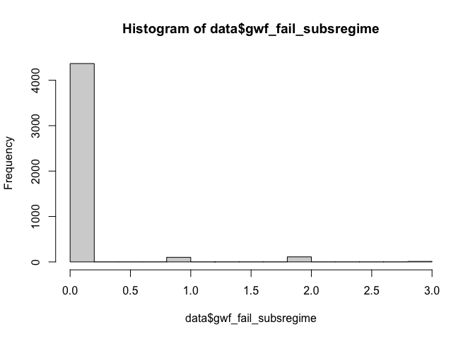
The data has 17 variables. The research is interested mainly in the “gwf_fail_subsregime” variable (Categorical variable marking the subsequent regime type), which has 4 responses gwf fail subs: Categorical variable marking the subsequent regime type • 1: subsequent regime is democracy • 2: subsequent regime is autocratic • 3: subsequent regime is warlord, foreign-occupied or ceases to exist • 0: no regime failure at duration time t; and regime still in power when the data coded in 2010
Examining the response varibale shows us that the value 0 is the highist (which represents “no regime failure of the autocratic regime”), which make the data skewed. Additionally, I am interested in the aftermath situation of the ended autocratic regimes.
table(data$gwf_fail_subsregime)

##
##    0    1    2    3
## 4368  101  111   11

hist(data$gwf_fail_subsregime)
 Therefore I am going to delete the observations that refere to “regime
still in power”, and which has 0 value.
Therefore I am going to delete the observations that refere to “regime
still in power”, and which has 0 value.
library(dplyr)
data1 <- filter(data, gwf_fail_subsregime %in% c("1", "2", "3"))
The potential explantory variables which would have, at least
theoritcally, statistical significance are: gwf_spell: Time-invariant
duration of autocratic regime gwf_fail_violent: Categorical variable
marking the level of violence during the autocratic regime failure event
gwf_regimetype: categorical variable of autocratic regime type
(pre-existing regime) gwf_fail_type:Categorical variable marking how
the autocratic regime ends gwf_party: Binary indicator of party regime
type
gwf_personal: Binary indicator of personal regime type
gwf_military: Binary indicator of military regime type
gwf_monarch: Binary indicator of monarchy regime type
The gwf_regimetype & gwf_fail_type could be useful (theoretically), however, they have many categories which would complecate the model (10 each)
table(data1$gwf_regimetype)

##
##       indirect military                military       military-personal
##                       6                      47                      23
##                monarchy               oligarchy             party-based
##                      12                       4                      35
##          party-military          party-personal party-personal-military
##                       6                      11                       2
##                personal
##                      77

table(data1$gwf_fail_type)

##
##  1  2  3  4  5  6  7  8  9
## 10 28 31 38 77 17 10  7  5
Therefore, I will not include these two variables in the model. At the same time, the dummy variables of personal and military regimes type are included, which adress part of the autocratic regimes. Additionally the variable of the level of violence during the failure of the autocratic regime partly adresses the way in which regime fails (violently or not)
Yet, gwf_fail_violent have 4 cateogries • 1: no deaths • 2: 1-25 deaths • 3: 26-1000 deaths • 4: >1000 • 0: regime still in power on December 31, 2010 I need to make it dummy and change the values, with 1 if there is death (the transation is violent), and 0 if there is no death
data1$gwf_fail_violent [data1$gwf_fail_violent == 2] <- 2
data1$gwf_fail_violent [data1$gwf_fail_violent == 3] <- 2
data1$gwf_fail_violent [data1$gwf_fail_violent == 4] <- 2
data1$gwf_fail_violent [data1$gwf_fail_violent == 1] <- 0
data1$gwf_fail_violent [data1$gwf_fail_violent == 2] <- 1
table(data1$gwf_fail_violent)

##
##   0   1
## 125  98
Finally I am going to rename the variables that I am interested in for my model
library(haven)

data1 <- data1 %>% dplyr::rename(duration = gwf_spell, subregime = gwf_fail_subsregime, violent = gwf_fail_violent, party = gwf_party,
                 personal = gwf_personal, military = gwf_military)
str(data1)

## tibble [223 × 17] (S3: tbl_df/tbl/data.frame)
##  $ cowcode       : num [1:223] 40 41 41 41 41 41 41 41 42 42 ...
##  $ year          : num [1:223] 1959 1946 1956 1986 1988 ...
##  $ gwf_country   : chr [1:223] "Cuba" "Haiti" "Haiti" "Haiti" ...
##  $ gwf_casename  : chr [1:223] "Cuba 52-59" "Haiti 41-46" "Haiti 50-56" "Haiti 57-86" ...
##  $ gwf_startdate : chr [1:223] "19270" "15102" "18541" "14/06/1957" ...
##  $ gwf_enddate   : chr [1:223] "21551" "17107" "20801" "31595" ...
##  $ duration      : num [1:223] 7 5 6 29 2 2 3 5 32 2 ...
##  $ gwf_duration  : num [1:223] 7 5 6 29 2 2 3 5 32 2 ...
##  $ gwf_fail      : num [1:223] 1 1 1 1 1 1 1 1 1 1 ...
##  $ subregime     : num [1:223] 2 1 2 2 2 1 1 1 2 2 ...
##  $ gwf_fail_type : num [1:223] 6 4 4 4 5 3 7 6 5 6 ...
##  $ violent       : num [1:223] 1 1 1 1 1 0 0 1 0 1 ...
##  $ gwf_regimetype: chr [1:223] "personal" "personal" "personal" "personal" ...
##  $ party         : num [1:223] 0 0 0 0 0 0 0 0 0 0 ...
##  $ personal      : num [1:223] 1 1 1 1 0 0 0 1 1 0 ...
##  $ military      : num [1:223] 0 0 0 0 1 1 1 0 0 1 ...
##  $ gwf_monarch   : num [1:223] 0 0 0 0 0 0 0 0 0 0 ...
we can see that R is reading the variable as integer, so we need to convert them to factor. However, no need for factorizing the duration, which is a counter variable
data1 <- data1 %>%
  mutate(subregime = as_factor(subregime), violent = as_factor(violent),
         party = as_factor(party), personal = as_factor(personal), military = as_factor(military))
##Visualizing the variables
Since we have 3 dummy variables, we can use plot function to visualize the relation between the response (subregime) and the explantory variables:
plot(data1$subregime, data1$violent, main = "Subsequent Regime Type & the Violent/Non Violent Transition", xlab = "Subregime Nature", ylab = "Non Violent/Violent", col = c("white","red"))
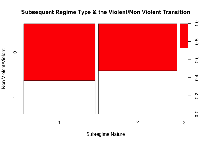 We can see that the violent transition is more represent in the 3
reponse possibility of the subsequent regime, this result is logical
giving that the third case represents “warlord, foreign-occupied or
ceases to exist”. In the same vein, the transition into “democracy” as
in the case number 1 is the less violent, while the transition to
autocratic regime is relatively violent.
We can see that the violent transition is more represent in the 3
reponse possibility of the subsequent regime, this result is logical
giving that the third case represents “warlord, foreign-occupied or
ceases to exist”. In the same vein, the transition into “democracy” as
in the case number 1 is the less violent, while the transition to
autocratic regime is relatively violent.
plot(data1$subregime, data1$military, main = "Subsequent Regime Type & the Military Autocratic Regime", xlab = "Subregime Nature", ylab = "Non Military/Military", col = c("white","green"))
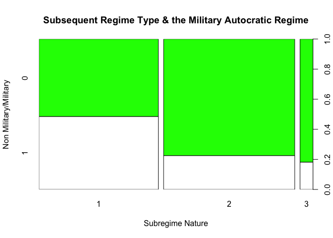 We can infere from the plot above that the military nature of the
autocratic regime prevent the country from sliding into a situation of
warlords or occupation after the change of the autocratic regime. But
what is puzzling here is that the military regime nature seems to
present more on the case of transition into democracy more that
autocratic case.
We can infere from the plot above that the military nature of the
autocratic regime prevent the country from sliding into a situation of
warlords or occupation after the change of the autocratic regime. But
what is puzzling here is that the military regime nature seems to
present more on the case of transition into democracy more that
autocratic case.
plot(data1$subregime, data1$personal, main = "Subsequent Regime Type & the Perosnal Autocratic Regime", xlab = "Subregime Nature", ylab = "Non Perosnal/Personal", col = c("white","blue"))
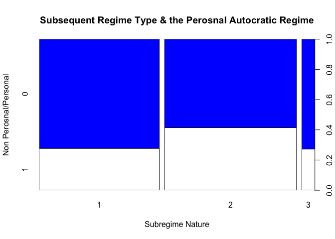 The personalist nature of the regime seems to present more in the cases
of transition to autocratic regimes (response case 2), more than in the
response case 1, which represents the transition into democratic
regimes.
The personalist nature of the regime seems to present more in the cases
of transition to autocratic regimes (response case 2), more than in the
response case 1, which represents the transition into democratic
regimes.
3. Methods
Since my response variable is categorical, with more than two catogories, I will use multinominal regression model, using nnet packcage. The multinominal model has two main assumptions: 1. The categories should be mutually exclusive and exhaustive Which seems to be the case for the three catgories that we have (1.democracy, 2.autocratic, 3.warlord foreign-occupied or ceases to exis) 2. Independence of irrelevant alternatives (IIA): It seems that this assumption is not violated. The tranisition process is not a choicable, rather it is self-realized in which the proportion of choosing one of the two alternatives is not change with the introduction of a third alternative. All alternatives of possible subsequent regimes are theoretically possible and known to the actors, but the path of the transition is not effected by their theoritical existence.
For nunning the model with subregime as the response variable, I will choose democracy as the reference category. Democracy is considered to be the ideal and reference model for democratization and regime transition theories, and also it represents one end of the continuum (of the categories) which make it easier to interpret the coefficients. It is better than the other end of the continuum which is cateogry 3 (warlord, foreign-occupied or ceases to exist) because it has more observation (101 to 11), and that would help reducing standard error and decreasing confidence interval width of other coefficients.
In the light of the hypotheses the possible models are as below:
Model1
model1 <- nnet::multinom(relevel(subregime , ref = "1") ~  duration + violent , data1)

## # weights:  12 (6 variable)
## initial  value 244.990540
## iter  10 value 185.425351
## final  value 185.415096
## converged

tab_model(model1, title = "Subsequent Regime", p.style = "a")
| relevel(subregime, ref = “1”) | |||
|---|---|---|---|
| Predictors | Odds Ratios | CI | Response |
| (Intercept) | 1.02 | 0.67 – 1.57 | 2 |
| duration | 0.99 | 0.98 – 1.01 | 2 |
| violent \[1\] | 1.59 | 0.91 – 2.76 | 2 |
| (Intercept) | 0.03 \*\*\* | 0.01 – 0.12 | 3 |
| duration | 1.02 | 0.99 – 1.04 | 3 |
| violent \[1\] | 4.41 \* | 1.09 – 17.79 | 3 |
| Observations | 223 | ||
| R2 Nagelkerke | 0.055 | ||
| - p<0.05 \*\* p<0.01 \*\*\* p<0.001 | |||
Model2
model2 <- nnet::multinom(relevel(subregime , ref = "1") ~  duration + violent + personal, data1)

## # weights:  15 (8 variable)
## initial  value 244.990540
## iter  10 value 184.065706
## final  value 183.731789
## converged

tab_model(model2, title = "Subsequent Regime", p.style = "a")
| relevel(subregime, ref = “1”) | |||
|---|---|---|---|
| Predictors | Odds Ratios | CI | Response |
| (Intercept) | 0.83 | 0.52 – 1.35 | 2 |
| duration | 0.99 | 0.98 – 1.01 | 2 |
| violent \[1\] | 1.51 | 0.87 – 2.64 | 2 |
| personal \[1\] | 1.71 | 0.95 – 3.09 | 2 |
| (Intercept) | 0.03 \*\*\* | 0.01 – 0.13 | 3 |
| duration | 1.02 | 0.99 – 1.05 | 3 |
| violent \[1\] | 4.38 \* | 1.08 – 17.74 | 3 |
| personal \[1\] | 1.07 | 0.25 – 4.65 | 3 |
| Observations | 223 | ||
| R2 Nagelkerke | 0.072 | ||
| - p<0.05 \*\* p<0.01 \*\*\* p<0.001 | |||
Model3
model3 <- nnet::multinom(relevel(subregime , ref = "1") ~  duration + violent + military, data1)

## # weights:  15 (8 variable)
## initial  value 244.990540
## iter  10 value 175.721134
## final  value 175.674340
## converged

tab_model(model3, title = "Subsequent Regime", p.style = "a")
| relevel(subregime, ref = “1”) | |||
|---|---|---|---|
| Predictors | Odds Ratios | CI | Response |
| (Intercept) | 2.14 \*\* | 1.22 – 3.76 | 2 |
| duration | 0.98 \* | 0.96 – 1.00 | 2 |
| violent \[1\] | 1.38 | 0.77 – 2.46 | 2 |
| military \[1\] | 0.25 \*\*\* | 0.13 – 0.47 | 2 |
| (Intercept) | 0.06 \*\*\* | 0.01 – 0.25 | 3 |
| duration | 1.01 | 0.98 – 1.04 | 3 |
| violent \[1\] | 4.04 | 0.99 – 16.41 | 3 |
| military \[1\] | 0.32 | 0.06 – 1.71 | 3 |
| Observations | 223 | ||
| R2 Nagelkerke | 0.152 | ||
| - p<0.05 \*\* p<0.01 \*\*\* p<0.001 | |||
To compare between the models:
tab_model(model1, model2, model3, title = "Subsequent Regime", p.style = "a")
| relevel(subregime, ref = “1”) | relevel(subregime, ref = “1”) | relevel(subregime, ref = “1”) | |||||||
|---|---|---|---|---|---|---|---|---|---|
| Predictors | Odds Ratios | CI | Response | Odds Ratios | CI | Response | Odds Ratios | CI | Response |
| (Intercept) | 1.02 | 0.67 – 1.57 | 2 | 0.83 | 0.52 – 1.35 | 2 | 2.14 \*\* | 1.22 – 3.76 | 2 |
| (Intercept) | 1.02 | 0.67 – 1.57 | 2 | 0.83 | 0.52 – 1.35 | 2 | 0.06 \*\*\* | 0.01 – 0.25 | 3 |
| (Intercept) | 1.02 | 0.67 – 1.57 | 2 | 0.03 \*\*\* | 0.01 – 0.13 | 3 | 2.14 \*\* | 1.22 – 3.76 | 2 |
| (Intercept) | 1.02 | 0.67 – 1.57 | 2 | 0.03 \*\*\* | 0.01 – 0.13 | 3 | 0.06 \*\*\* | 0.01 – 0.25 | 3 |
| duration | 0.99 | 0.98 – 1.01 | 2 | 0.99 | 0.98 – 1.01 | 2 | 0.98 \* | 0.96 – 1.00 | 2 |
| duration | 0.99 | 0.98 – 1.01 | 2 | 0.99 | 0.98 – 1.01 | 2 | 1.01 | 0.98 – 1.04 | 3 |
| duration | 0.99 | 0.98 – 1.01 | 2 | 1.02 | 0.99 – 1.05 | 3 | 0.98 \* | 0.96 – 1.00 | 2 |
| duration | 0.99 | 0.98 – 1.01 | 2 | 1.02 | 0.99 – 1.05 | 3 | 1.01 | 0.98 – 1.04 | 3 |
| violent \[1\] | 1.59 | 0.91 – 2.76 | 2 | 1.51 | 0.87 – 2.64 | 2 | 1.38 | 0.77 – 2.46 | 2 |
| violent \[1\] | 1.59 | 0.91 – 2.76 | 2 | 1.51 | 0.87 – 2.64 | 2 | 4.04 | 0.99 – 16.41 | 3 |
| violent \[1\] | 1.59 | 0.91 – 2.76 | 2 | 4.38 \* | 1.08 – 17.74 | 3 | 1.38 | 0.77 – 2.46 | 2 |
| violent \[1\] | 1.59 | 0.91 – 2.76 | 2 | 4.38 \* | 1.08 – 17.74 | 3 | 4.04 | 0.99 – 16.41 | 3 |
| (Intercept) | 0.03 \*\*\* | 0.01 – 0.12 | 3 | 0.83 | 0.52 – 1.35 | 2 | 2.14 \*\* | 1.22 – 3.76 | 2 |
| (Intercept) | 0.03 \*\*\* | 0.01 – 0.12 | 3 | 0.83 | 0.52 – 1.35 | 2 | 0.06 \*\*\* | 0.01 – 0.25 | 3 |
| (Intercept) | 0.03 \*\*\* | 0.01 – 0.12 | 3 | 0.03 \*\*\* | 0.01 – 0.13 | 3 | 2.14 \*\* | 1.22 – 3.76 | 2 |
| (Intercept) | 0.03 \*\*\* | 0.01 – 0.12 | 3 | 0.03 \*\*\* | 0.01 – 0.13 | 3 | 0.06 \*\*\* | 0.01 – 0.25 | 3 |
| duration | 1.02 | 0.99 – 1.04 | 3 | 0.99 | 0.98 – 1.01 | 2 | 0.98 \* | 0.96 – 1.00 | 2 |
| duration | 1.02 | 0.99 – 1.04 | 3 | 0.99 | 0.98 – 1.01 | 2 | 1.01 | 0.98 – 1.04 | 3 |
| duration | 1.02 | 0.99 – 1.04 | 3 | 1.02 | 0.99 – 1.05 | 3 | 0.98 \* | 0.96 – 1.00 | 2 |
| duration | 1.02 | 0.99 – 1.04 | 3 | 1.02 | 0.99 – 1.05 | 3 | 1.01 | 0.98 – 1.04 | 3 |
| violent \[1\] | 4.41 \* | 1.09 – 17.79 | 3 | 1.51 | 0.87 – 2.64 | 2 | 1.38 | 0.77 – 2.46 | 2 |
| violent \[1\] | 4.41 \* | 1.09 – 17.79 | 3 | 1.51 | 0.87 – 2.64 | 2 | 4.04 | 0.99 – 16.41 | 3 |
| violent \[1\] | 4.41 \* | 1.09 – 17.79 | 3 | 4.38 \* | 1.08 – 17.74 | 3 | 1.38 | 0.77 – 2.46 | 2 |
| violent \[1\] | 4.41 \* | 1.09 – 17.79 | 3 | 4.38 \* | 1.08 – 17.74 | 3 | 4.04 | 0.99 – 16.41 | 3 |
| personal \[1\] | 1.71 | 0.95 – 3.09 | 2 | ||||||
| personal \[1\] | 1.07 | 0.25 – 4.65 | 3 | ||||||
| military \[1\] | 0.25 \*\*\* | 0.13 – 0.47 | 2 | ||||||
| military \[1\] | 0.32 | 0.06 – 1.71 | 3 | ||||||
| Observations | 223 | 223 | 223 | ||||||
| R2 Nagelkerke | 0.055 | 0.072 | 0.152 | ||||||
| - p<0.05 \*\* p<0.01 \*\*\* p<0.001 | |||||||||
#install.packages("lmtest")
library(lmtest)

## Loading required package: zoo

##
## Attaching package: 'zoo'

## The following objects are masked from 'package:base':
##
##     as.Date, as.Date.numeric

lrtest(model1, model2, model3)

## Likelihood ratio test
##
## Model 1: relevel(subregime, ref = "1") ~ duration + violent
## Model 2: relevel(subregime, ref = "1") ~ duration + violent + personal
## Model 3: relevel(subregime, ref = "1") ~ duration + violent + military
##   #Df  LogLik Df   Chisq Pr(>Chisq)
## 1   6 -185.41
## 2   8 -183.73  2  3.3666     0.1858
## 3   8 -175.67  0 16.1149     <2e-16 ***
## ---
## Signif. codes:  0 '***' 0.001 '**' 0.01 '*' 0.05 '.' 0.1 ' ' 1
The test shows us again that the third model seems to have the best likelihood ratio among the three models.
4. Results
After doing these tests, it is clear that the third model is the best among our models to predict the subsequent regime nature. The third model does not only have more liklihood ratio, but it also represent an interesing results for the academia and the related literature.
tab_model(model3, title = "Subsequent Regime", p.style = "a")
| relevel(subregime, ref = “1”) | |||
|---|---|---|---|
| Predictors | Odds Ratios | CI | Response |
| (Intercept) | 2.14 \*\* | 1.22 – 3.76 | 2 |
| duration | 0.98 \* | 0.96 – 1.00 | 2 |
| violent \[1\] | 1.38 | 0.77 – 2.46 | 2 |
| military \[1\] | 0.25 \*\*\* | 0.13 – 0.47 | 2 |
| (Intercept) | 0.06 \*\*\* | 0.01 – 0.25 | 3 |
| duration | 1.01 | 0.98 – 1.04 | 3 |
| violent \[1\] | 4.04 | 0.99 – 16.41 | 3 |
| military \[1\] | 0.32 | 0.06 – 1.71 | 3 |
| Observations | 223 | ||
| R2 Nagelkerke | 0.152 | ||
| - p<0.05 \*\* p<0.01 \*\*\* p<0.001 | |||
However, there are no statistically significant results for response 3, which is the case of having a civil war and warlords states in the subsequent regime.The absance of statistically significant results for response 3, could be due to the limited numbers of observations that we have in response 3; just 3 observation.
table(data1$subregime)

##
##   1   2   3
## 101 111  11
we can also develop a confusion matrix to test how well our model does in predicting the target variable.
#install.packages("caret")
library(caret)

## Loading required package: lattice

library(e1071)
pred <- predict(model3)
caret::confusionMatrix(data=pred, data1$subregime)

## Confusion Matrix and Statistics
##
##           Reference
## Prediction  1  2  3
##          1 61 29  4
##          2 40 82  7
##          3  0  0  0
##
## Overall Statistics
##
##                Accuracy : 0.6413
##                  95% CI : (0.5745, 0.7042)
##     No Information Rate : 0.4978
##     P-Value [Acc > NIR] : 1.096e-05
##
##                   Kappa : 0.3116
##
##  Mcnemar's Test P-Value : 0.005201
##
## Statistics by Class:
##
##                      Class: 1 Class: 2 Class: 3
## Sensitivity            0.6040   0.7387  0.00000
## Specificity            0.7295   0.5804  1.00000
## Pos Pred Value         0.6489   0.6357      NaN
## Neg Pred Value         0.6899   0.6915  0.95067
## Prevalence             0.4529   0.4978  0.04933
## Detection Rate         0.2735   0.3677  0.00000
## Detection Prevalence   0.4215   0.5785  0.00000
## Balanced Accuracy      0.6667   0.6595  0.50000
The model has 64.1% accuray in prediction the observations, which is a modest value. From the matrix, we can see again that our model, model3, have serious shortages in predicting the possibility of third response case (warlord, foreign-occupied or ceases to exist), which as mentioned, could be due to the limited numbers of response observations (just 11 out of 223)
5. Conclusion
The final results of the chosen model (model3) are academically interesting and somehow counterintuitive, even though the statistical significant of the model seems to be modest. The modest statistical significant is mainly due to the limited number of observations, in particular for the personal autocratic regime, which is due to the limited number of the samples (changed autocratic regimes). Going back to the three hypotheses; the duration or age of the autocratic regime has impact on the subsequent regime nature, though the odd is too small to be considered; the personalist regime nature does not seem to have impact on the subsequent regime, which could be due to statistical shortages and small sampling; while the military regime nature seems to impact the subsequent regime nature, what was counterintuitive is that the impact is positive on the possibilities of establishing a democratic regime after the autocratic regime collapses. This interesting result would contribute to the democratization and regime change theory, while at the same time represents a puzzle regarding the relation between military tutelage and democracy. Hence, future studies could focus in detail on the correlation between military regimes and the possibilities of democratization beyond simple assumptions.
Co-Director
Global Governance Centre
Professor
International Relations and Political Science
President
Global Governance Research Centre Consortium
International institutions and political networks.