No Safe Place, Analyzing attacks against aid workers
Swetha Ramachandran - Statistics for International Relations Research II
Introduction
Attacks against aid workers have gradually witnessed an upward trend in the last decade. The number of victims increased to 313 in 2017 and to over 400 in 2018, marking an all-time high in the last 5 years. It speaks to the difficulty in keeping staff secure in the conflict-affected and volatile environments where these attacks take place (Aid Worker Security Report, 2019). Currently, there is little to no systematic analysis about the modalities of these attacks: what methods are used to attack aid workers, where, how, are internationals more impacted than local staff etc. By analyzing the Aid Worker Security Database (AWSD), this blog post answers the following question: “What factors predict the probability of”how" attacks against aid workers are carried out (or means of attack)?". Simply put, I am trying to explain a conditional probability question: Given that an attack against aid workers has already happened, what factors explain “how” it took place? I specifically study the following means of attack: Bombs, Kidnapping, Shooting, Bodily harm and test the following hypotheses:
H1: There exists a positive relationship between attack context (whether crossfire, mob, or individual attack), place of attack (whether at office/home) and means of attack.
H2: There exists a positive association between presence of national staff and means of attack.
Preliminary findings using multinomial logit model suggest that the attack context, place and national/international staff status emerge statistically significant, even though the direction varies depending on teh categories within these variables.
Data
Overview:
The dataset I will be using is called the “Aid Worker Security Database (AWSD)”. It records major attacks against humanitarian workers from 1997-present (2021) and has 3115 observations in total across 43 variables. To be recorded in the AWSD, the attack would first have to entail “major” violence, in which victims were killed, kidnapped, or seriously injured as a result. Additionally, they would have to be personnel of a humanitarian organization (including staff, volunteers, community outreach workers, or public sector employees supported by an international humanitarian agency or donor as part of an emergency response). For this post, I will be using the following variables from AWSD:
Dependent Variable (DV):
- Means of attack
- Categorical variable with 4 categories: Bodily harm, Bombs, Kidnapping, Shooting
Independent Variables (IV):
- Place/Location of attack
- Categorical variable with 3 categories: Home, Public, Work
- Attack context
- Categorical variable with 4 categories: Ambush, Combat/Crossfire, Individual attack, Mob
- UN
- Dummy variable, 0 = No UN worker involved in the attack, 1 = Atleast 1 UN worker involved in the attack
- Total nationals
- Discrete variable indicating number of national staff involved in the attack across organizations
- Total internationals:
- Discrete variable indicating number of international staff involved in the attack across organizations
Cleaning:
The data could not be used directly in the original format and necessitated cleaning using the following steps:
Variable transformations: In the original dataset, vars means of attack, attack location and attack context are categorical variables, each with 7+ categories each. I combined conceptually similar categories to transform them into categorical variables with 3-4 categories each. In addition to facilitating anlaysis, this transformation also helps circumvent issues of perfect separation. Also, a new variable called UN_dummy was created for analysis.
Recoding: “Unknowns” were recoded as “NAs”. This is because the “Unknown” label can be misunderstood as not knowing where or how to attack when it’s actually a missing data problem.
Data type: Factor variables converted into correct format.
Missing data checks:
Using the “Naniar” package in R, we visually inspect the data for
missing observations:
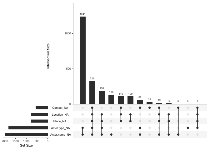
The “upset” option allows us to study combination of missing-ness.
We notice that 1241 observations are missing for actor type and name.
This is acceptable given that we won’t be focussing on the two
variables. Other missing values are relatively smaller as a proportion
of the total sample size and raise no major concerns. Given the nature
of data collection (self-reporting by aid organizations) and the
logistical difficulties in determining certain aspects of the attack
(such as which group perpetrated it), I will assume that the data is
“Missing not at random (or MNAR)”. While there is a risk that MNAR will
introduce bias into the estiamtes, this problem is invariable given the
type of dataset we are dealing with.
Now we proceed to describing the dataset using visuals.
Description:
Provided below are the summary statistics for variables of interest:
## [1] "<table class=\"Rtable1\">\n<thead>\n<tr>\n<th class='rowlabel firstrow lastrow'></th>\n<th class='firstrow lastrow'><span class='stratlabel'>Overall<br><span class='stratn'>(N=3115)</span></span></th>\n</tr>\n</thead>\n<tbody>\n<tr>\n<td class='rowlabel firstrow'><span class='varlabel'>UN_dummy</span></td>\n<td class='firstrow'></td>\n</tr>\n<tr>\n<td class='rowlabel'>Mean (SD)</td>\n<td>0.219 (0.414)</td>\n</tr>\n<tr>\n<td class='rowlabel lastrow'>Median [Min, Max]</td>\n<td class='lastrow'>0 [0, 1.00]</td>\n</tr>\n<tr>\n<td class='rowlabel firstrow'><span class='varlabel'>Total.nationals</span></td>\n<td class='firstrow'></td>\n</tr>\n<tr>\n<td class='rowlabel'>Mean (SD)</td>\n<td>1.62 (2.11)</td>\n</tr>\n<tr>\n<td class='rowlabel lastrow'>Median [Min, Max]</td>\n<td class='lastrow'>1.00 [0, 49.0]</td>\n</tr>\n<tr>\n<td class='rowlabel firstrow'><span class='varlabel'>Total.internationals</span></td>\n<td class='firstrow'></td>\n</tr>\n<tr>\n<td class='rowlabel'>Mean (SD)</td>\n<td>0.252 (0.845)</td>\n</tr>\n<tr>\n<td class='rowlabel lastrow'>Median [Min, Max]</td>\n<td class='lastrow'>0 [0, 15.0]</td>\n</tr>\n<tr>\n<td class='rowlabel firstrow'><span class='varlabel'>Means</span></td>\n<td class='firstrow'></td>\n</tr>\n<tr>\n<td class='rowlabel'>Bodily harm</td>\n<td>618 (19.8%)</td>\n</tr>\n<tr>\n<td class='rowlabel'>Bombs</td>\n<td>447 (14.3%)</td>\n</tr>\n<tr>\n<td class='rowlabel'>Kidnapping</td>\n<td>730 (23.4%)</td>\n</tr>\n<tr>\n<td class='rowlabel'>Shooting</td>\n<td>900 (28.9%)</td>\n</tr>\n<tr>\n<td class='rowlabel lastrow'>Missing</td>\n<td class='lastrow'>420 (13.5%)</td>\n</tr>\n<tr>\n<td class='rowlabel firstrow'><span class='varlabel'>Place</span></td>\n<td class='firstrow'></td>\n</tr>\n<tr>\n<td class='rowlabel'>Home</td>\n<td>240 (7.7%)</td>\n</tr>\n<tr>\n<td class='rowlabel'>Public</td>\n<td>1509 (48.4%)</td>\n</tr>\n<tr>\n<td class='rowlabel'>Work</td>\n<td>601 (19.3%)</td>\n</tr>\n<tr>\n<td class='rowlabel lastrow'>Missing</td>\n<td class='lastrow'>765 (24.6%)</td>\n</tr>\n<tr>\n<td class='rowlabel firstrow'><span class='varlabel'>Context</span></td>\n<td class='firstrow'></td>\n</tr>\n<tr>\n<td class='rowlabel'>Ambush</td>\n<td>1060 (34.0%)</td>\n</tr>\n<tr>\n<td class='rowlabel'>Combat/Crossfire</td>\n<td>393 (12.6%)</td>\n</tr>\n<tr>\n<td class='rowlabel'>Individual attack</td>\n<td>647 (20.8%)</td>\n</tr>\n<tr>\n<td class='rowlabel'>Mob</td>\n<td>463 (14.9%)</td>\n</tr>\n<tr>\n<td class='rowlabel lastrow'>Missing</td>\n<td class='lastrow'>552 (17.7%)</td>\n</tr>\n</tbody>\n</table>\n"
We notice that our main categorical variables are well spread across
the different categories, except for the Place var which has ~50% of
observations coded as “Public” and only around ~8% at home. However,
combining categories beyond this level to make the spread more equitable
does not make theoretical sense, so we will retain it as is. Missing
values are mostly below 20%, except for the variable “Place”, which is
~25%.
Now we graphically visualize our 3 main categorical variables, Means of attack (DV), Place (IV) and Context (IV), to get a sense of how they relate to each other.
Figure 1.0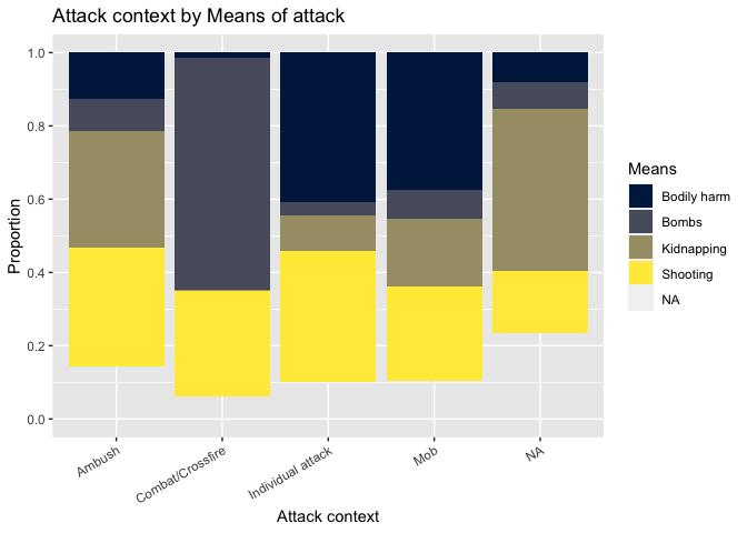
Figure 2.0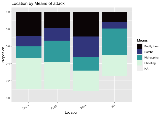
A final visual to identify countries in which the attacks were perpetuated:
Figure 3.0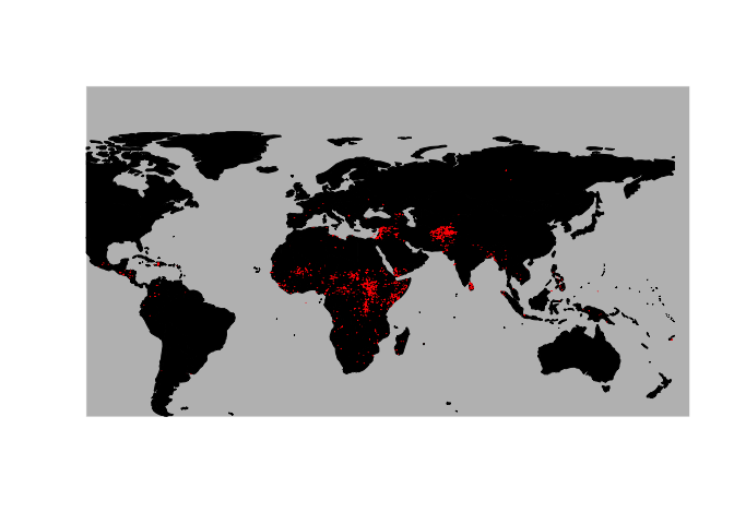
From the map, it looks like most attacks took place in the
continents of Africa, Middle East and parts of South Asia, and more
specifically in Afghanistan, around Syria, South Sudan, Horn of Africa,
DRC and CAR. The geography is not of direct relevance for the hypotheses
that we are testing, but provides some contexual information
nonetheless.
Potential data issues:
It is well acknowledged that the AWSD is severely under-representative of the true numbers, as not all aid workers report violent incidents against them, especially when it comes to sexual violence and exploitation. One must also note that perpetrators from within the aid space are not recorded (i.e. if an aid worker was sexually exploited by another staff member, the dataset would not record that). Also, organizations self-report these attacks, which can lead to heavy biases in reporting.
Methods
To analyze the AWSD, I will be using a “multinomial logistic” regression model. The rationale is that the DV (Means of attack) is an unordered response variable with 4 categories. So we use the model to predict the probabilities of the different possible outcomes of a categorically distributed dependent variable, given a set of independent variables (which may be dummy, categorical, discrete etc). To use multinomial logit, we need to meet 2 assumptions:
Mutually exclusive and exhaustive: This assumption is usually driven by theory rather than a specific statistical test. Our DV is indeed mutually exclusive (i.e. response belongs to only one category). This was apparent during the cleaning process when categories were collapsed as all responses belonged to only one category or another. On the question of whether the DV is exhaustive (that it covers all possibilities), this can be debated. The current conceptualization covers the broad attack means of shooting, kidnapping, bodily harm and bombs, and one can posit that most means can easily qualify under these categories. Keeping this as a rationale, we will proceed with the understanding the the exhaustive assumption is also met.
Independence of irrelevant alternatives (IIA) The IIA assumption means that adding or deleting alternative outcome categories does not affect the odds among the remaining outcomes. We will get back to this test once the models are run in the results section below. If the IIA is violated, options to correct for it include Heteroskedastic multinomial logit, multinomial probit or nested logit.
Models
Model 1 (nested) = DV: Means, IVs: Context, Location, UN Dummy Model 2 (complex = DV: Means, IVs: Context, Location, UN Dummy, Total nationals, Total internationals
We now run these models in the next section, analyze their fit, check for marginal effects and finally do the standard tests for multicollinearity, heterskedasticity, outliers.
Results
Running the models
| Bombs | Kidnapping | Shooting | Bombs | Kidnapping | Shooting | |
| Model 1 | Model 2 | |||||
| Constant | -0.256 (0.365) | 1.604\*\*\* (0.316) | 1.460\*\*\* (0.239) | -0.838\*\* (0.379) | 1.148\*\*\* (0.327) | 1.339\*\*\* (0.253) |
| ContextCombat/Crossfire | 4.116\*\*\* (0.532) | -1.931\*\* (0.881) | 1.956\*\*\* (0.528) | 4.348\*\*\* (0.534) | -1.744\*\* (0.882) | 1.985\*\*\* (0.529) |
| ContextIndividual attack | -2.032\*\*\* (0.277) | -2.688\*\*\* (0.225) | -1.348\*\*\* (0.166) | -1.753\*\*\* (0.282) | -2.483\*\*\* (0.230) | -1.291\*\*\* (0.168) |
| ContextMob | -1.510\*\*\* (0.304) | -2.109\*\*\* (0.264) | -1.481\*\*\* (0.214) | -1.730\*\*\* (0.317) | -2.259\*\*\* (0.273) | -1.475\*\*\* (0.215) |
| PlacePublic | -0.082 (0.335) | -0.600\*\* (0.296) | -0.547\*\*\* (0.212) | -0.284 (0.343) | -0.813\*\*\* (0.301) | -0.580\*\*\* (0.213) |
| PlaceWork | 0.379 (0.323) | -0.075 (0.262) | -0.519\*\* (0.206) | -0.005 (0.336) | -0.409 (0.270) | -0.580\*\*\* (0.209) |
| UN\_dummy | 0.151 (0.205) | -0.219 (0.172) | 0.240 (0.146) | 0.037 (0.210) | -0.296\* (0.176) | 0.195 (0.147) |
| Total.nationals | 0.410\*\*\* (0.060) | 0.352\*\*\* (0.057) | 0.112\* (0.060) | |||
| Total.internationals | 0.465\*\*\* (0.111) | 0.459\*\*\* (0.103) | -0.009 (0.116) | |||
| AIC | 4689.778 | 4689.778 | 4689.778 | 4571.020 | 4571.020 | 4571.020 |
| ***p < .01; **p < .05; *p < .1 | ||||||
Interpretation (highlights):
“Bodily assault” is the reference category in our DV, “Ambush” for the Context (one of our IV) and “Home” for Place var (also IV).
For the Context var, we note statistical significance and similarity in coefficient sign and magnititude across both models. The log odds of being attacked by bodily assault vs. bombs will increase by 4.1 if moving from ambush to combat/crossfire in model 1. This number slightly increases to 4.4 in model 2. Similarly, for instance, the log odds of being attacked by bodily assault vs. kidnapping will decrease by 2.7 if moving from ambush to individual attack in model 1. The same interpretation logic applies for other coefficients.
For the Place var, we note interesting variations. The log odds of being attacked by bodily assault vs. kidnapping orbodily assault vs. shooting is negative and statistically significant when attack location changes from home to public across both models. When location changes from home to work, log odds of being attacked by bodily assault vs. shooting is statistically significant and decreases by 0.52 and 0.58 in mode1 and 2 respectively.
UN_dummy var is not statistically significant at all, implying that whether or not a UN staff member is involved has no bearing on the means of attack
National v/s international status of staff members emerges significant in model 2. Both are positively associated with an increase in log odds of being attacked by bodily assault vs. kidnapping and bodily assault vs. bombs. The coefficients are in a small numeric range of 0.3-0.5.
Now let us check for the IIA assumption to see if the models still hold good.
IIA assumption
We can theoretically argue that adding or deleting another category in our DV “means” won’t drastically change the IIA assumption as the odds among the remaining outcomes won’t vary drastically. For instance, if we remove “shooting”, one could argue that the odds of “kidnapping” don’t have to change. Ofcourse, there is an implicit assumption that every attack that took place can be neatly defined into one category, so an attack is either shooting or kidnapping, but not both. While this can be debated in real life, the dataset has been constructed with exclusive categories only, so we can argue that IIA holds true. One can also run the “hmftest” from the mlogit package but this further investigation on R. For now, we can assume that IIA condition is met.
Analyzing the fit
For analyzing which model is better, we use the LRT (Likelihood ratio test):
## Likelihood ratio test
##
## Model 1: Means ~ Context + Place + UN_dummy
## Model 2: Means ~ Context + Place + UN_dummy + Total.nationals + Total.internationals
##   #Df  LogLik Df  Chisq Pr(>Chisq)
## 1  21 -2323.9
## 2  27 -2258.5  6 130.76  < 2.2e-16 ***
## ---
## Signif. codes:  0 '***' 0.001 '**' 0.01 '*' 0.05 '.' 0.1 ' ' 1
From the results, we see that the null hypothesis (that one should use nested model) would be rejected at nearly every significance level. We should instead use the complex model as it increases the accuracy of our model by a substantial amount. Now that we have chosen our complex model, we can calibrate the output of the model and examining all possible outcomes of our predictions (true positive, true negative, false positive, false negative) using a confusion matrix.
Accuracy
To ascertain the model’s accuracy, we will be creating a confusion matrix to see what percentage of the observations can be accurately predicted by our model.
I tried to run the confusion matrix but couldn’t mitigate the error message “Error in table(predicted, actual) : all arguments must have the same length”. With more time, I would be able to decode why the error remains. That being said the table function of both predicted and complex functions gives some sense of the accuracy:
##
## Bodily harm       Bombs  Kidnapping    Shooting
##         618         447         730         900

## pred
## Bodily harm       Bombs  Kidnapping    Shooting
##         685         301         439         621
Now we transition to marginal effects to see whether national/international staff status and UN dummy have more influences than we previously considered.
Marginal effects
We notice that for bombings and shootings, being a local and with
the UN puts the worker at a greater risk. This could be attributed to
the ‘self selection’ in that locals with the UN might be sent to more
challenging locations. Similarly, being international, but not with the
UN, can lead to a much greater incidence of kidnapping. This could be
explained by UN’s strict security protocols for expat staff which might
be missing in this case.
Finally, we conclude the analysis section with some diagnostic tests for our complex model.
Diagnostic tests
First we test for multicollinearity using the variance inflation factor (or VIF)
##                           GVIF Df GVIF^(1/(2*Df))
## Context              69.267787  3        2.026540
## Place                42.361203  2        2.551186
## UN_dummy              1.830375  1        1.352913
## Total.nationals       7.427332  1        2.725313
## Total.internationals  3.640216  1        1.907935
We see a high VIF for our categorical vars Context and Place. However, the potential reason could be that the proportion of cases in the reference category is small, meaning the indicator variables will necessarily have high VIFs (even if the categorical variable is not associated with other variables in the regression model).So we may consider reorganizing our categorical variables yet again and repeating the VIF test. Also broadly, logistic regression seems to assume that there is no severe multicollinearity among the explanatory variables anyways (since logit and linear models are driven by different sets of assumptions). This assertion is based on online resources.
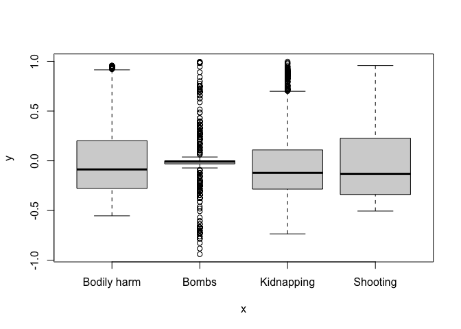
We now turn to evaluating outliers using boxplots. An outlier is
considered influential if its exclusion causes major changes in the
fitted regression function.
Here, we see a few points as outliers for nationals and
internationals, but this simply signifies the gravity of the attack
(larger the attack, more nationals/internationals impacted). While this
does raise a concern that some big attacks may be over-influencing our
estimates, it is a bit hard to account for which attacks should be
weighted more for instance. So these boxplots prompted me to
double-check the observations, but I choose to retain them in the
sample. These outliers could even provide more information upon further
investigation.
Finally, to detect heteroskedasticity, if we assume that the error terms are IID (identically and independently distributed), then they are automatically uncorrelated and homoscedastic. However, IID makes more sense for linear models than logit ones, which tend to follow a different set of assumptions. I’m unsure how to proceed with testing IID for multinomial logit models as the online resources suggest complicated models and tests. But a visual inspection of residuals and predicted values could help. Below is such a visual from our chosen “complex” model:
Conclusion
In summary, this blog model was a first attempt at answering “What factors predict the probability of means of attack against aid workers, given that an attack has taken place”? By using multinomial logit model, we find that the attack context, place and national/international staff status emerge statistically significant. Potential issues to resolve for future iterations include resolving the confusion matrix issue and running a test for IIA.
References
[1] Aid Worker Security Report (2021), Contending with threats to
humanitarian health workers in the age of epidemics
[2] Aid Worker
Security Dataset (2021)
[3] Dr. James Hollway, Course: Statistics
for IR slides (2021)
[4] Online resources, including but not
limited to: Stats.idre at UCLA, Cran.r-project manuals,
Stackoverflow.com, Github.io, Statology
Co-Director
Global Governance Centre
Professor
International Relations and Political Science
President
Global Governance Research Centre Consortium
International institutions and political networks.