When ICTs merge with governance in the 21st Century: an investigation of the association between e-governance advancement and governance quality of UN member states from 2003 to 2018
Chin Man Kwan - Statistics for International Relations Research II
- Introduction
- Literature Review
- Hypotheses
- Data and operationalisation
- Descriptive Statistics
- Methodology
- Results
- Robustness Check
- Conclusion
- Reference
- Appendix 1
- E-Government Development Index
- World Bank Control of Corruption Indicator
- World Bank Government Effectiveness Indicator
- World Bank Voice and Accountability Indicator
- GDP per capita in current USD
- FSI Demographic Pressure
- FSI Group Grievance
- FSI External Intervention
- FSI Refugees and IDPs
- V-Dem Women political empowerment index
Introduction
One of the most prominent and rapid technological developments in the 21st Century is information and communication technologies (ICTs), which are broadly defined as digital technologies which can “transmit, store, create, share or exchange information”, such as the Internet, broadcasting and telephone (UNESCO 2021). Subsequently, e-government, the usage of ICTs to develop more efficient government agencies, provide online government services and channels for citizens and business to interact with the government as well as permit open access to government data and facilitate innovative governance (United Nations 2021), has become more and more popular across countries[1].
To what extent has e-governance lived up to the expectation of improving governance quality around the world as two decades have elapsed in the 21st Century? Using UN member states as the unit of analysis, I will employ a linear mixed effects model to analyse the relationship between the level of e-governance and governance quality from 2003 to 2018 after controlling for other factors using a dataset generated by sources from the United Nation’s E-Government Development Index (EGDI), the World Bank’s Worldwide Governance Indicators (WGI) and the Quality of Governance time-series standard dataset by the University of Gothenburg (Teorell et al. 2021).
To briefly tease the results, the regression analysis result indicates that there is a lack of evidence to conclude that more advanced e-governance is associated with less corruption and better public service provision. As for improvement in government accountability, the result offers mixed support because there seems to be a non-linear relationship, namely, although initial advancement in e-governance is associated with more accountable government, once advancement reaches a certain point, the relationship may start to reverse.
This blog post’s structure is organised as follow. First, I will define what governance refers to in this analysis and review the literature on how e-governance is expected to assist in improving the quality of governance. Next, I will set up some hypotheses to investigate the relationship between e-governance level and governance performance according to the literature on e-governance. Afterwards, I will introduce the independent, control and dependent variables in terms of how they were operationalised, collected, measured, and potential issues in the data set. Then, I will introduce the statistical model which I will be using for the analysis, present and interpret the result while also checking for whether assumptions of the model used are grossly violated and perform several robustness checks on the result. The conclusion will summarise the findings, discuss the limitations and suggest further research directions on e-governance.
Literature Review
Defining governance
It is imperative to first define what governance means in this blog post for a coherent discussion and analysis in subsequent sections. Admittedly, the concept of (good) governance is difficult to be captured by a single definition, as Barthwal (2003) and Kaufmann et al. (2011) mention that there exist numerous definitions which vary on their scope, either broadly defining governance as a whole or specifically focusing on issues such as the rule of law and public sector management. But to provide a basis for this blog post’s analysis, I will adopt Kaufmann et al. (2011)’s definition of governance which consists of three major components, namely:
“(a) the process by which governments are selected, monitored and replaced; (b) the capacity of the government to effectively formulate and implement sound policies; and (c) the respect of citizens and the state for the institutions that govern economic and social interactions among them.” (p.222)
Note that this does not imply the definition proposed by Kaufmann et al. (2011) is necessarily superior than others. Rather, this definition is adopted because it serves better to evaluate whether advancement in e-governance is associated with improvement in governance quality given the envisioned benefits of developing e-governance repertoire by policy makers and scholars as mentioned in the next section. Moreover, narrowing down what governance means will be helpful for setting up more precise hypotheses which can be more easily operationalised and tested in the statistical analysis.
How e-governance is perceived to improve governance quality?
E-governance is envisioned by both policy makers and academics to improve the governance quality of a country in various ways. With regard to the policy-making world, e-governance is often envisioned to be beneficial in improving governance quality. For instance, the OECD argues e-governance can enhance the ability of member state to implement policies, provide government services more efficiently and effectively as well as standardising governance framework (OECD 2008). Likewise, the United Nations argue that e-government can be more than just facilitating public service provision since it can go as far as promoting democratic participation by citizens and even help developing countries to accelerate their developmental processes in improving the living standard of the people Smith and Teicher (2006). It seems therefore that policy makers are optimistic about the impact of e-governance in ameliorating the quality of life in different countries by fostering more effective and efficient governance.
Some scholars also agree that e-governance can be beneficial for enhancing governance quality. Studying the examples of e-governance initiatives put forward by various countries situated in different continents and different economic development levels, Barthwal (2003) and Singh et al. (2010) argue that more efficient public service provision to citizens, greater transparency, accountability, public participation in policy debates, access to government information and mitigating corruption are the potential benefits of adopting e-governance. Madon (2009) also mentions how e-governance projects in developing countries, mostly focused on digitalising administrative and service provision procedures of governments, are implemented by international development agencies such as the World Bank to advance the good governance agenda and thus mitigate the problem of underdevelopment. Therefore, promoting accountability and transparency of the government vis-a-vis the public, bolstering the effectiveness and efficiency of public services as well as reducing the level of corruption (i.e. abusing public power for private gains) are the some of the most widely proposed potential benefits of e-governance on governance quality in the literature.
There exist, however, numerous obstacles which hinder the ability of e-governance to improve the quality of governance as the above arguments have outlined. Apart from the enormous requirement for inputs to build up the infrastructures, Smith and Teicher (2006) mentions that even if bureaucracies have extensively digitalised their operations and public services provision, a lack of coordination and common operational standard among different government departments will constrain the ability of e-governance to deliver better governance coherently. Meanwhile, Madon (2009) mentions some citizens may be indifferent in benefiting from e-governance-provided service and welfare because of the low perceived relevance to daily life. Moreover, e-governance may also happen to be utilised by some national governments to achieve the opposite of the original aim, such as case studies on China and Jordan reveal that governments may actually use ICTs to tighten control over the citizens instead of empowering the mass for political participation (Madon 2009). Last but not least, the success of adopting ICTs to improve governance quality also depends partly on the presence of local intermediaries and their social networks to help reach out to the most vulnerable groups who may benefit the most from e-governance initiatives (Madon 2009).
From the above arguments, the effect of e-governance on improving governance quality should not be assumed to be a given. Rather, it is possible that obstacles in certain contexts may prevent the digitalisation and informatisation of governance from raising the living standards of the people. Nevertheless, while there have been a lot of studies which evaluate whether e-governance initiatives have improved the governance quality in specific countries (e.g. those cited in the previous paragraphs), there is yet to be a quantitative analysis to inquire the association between e-governance level and governance performance across a substantial amount of countries over a given period of time. This blog post thus aims to fill in this gap by using UN member states as the unit of analysis throughout the period 2003-18.
Hypotheses
Based on the review of arguments about how e-governance can promote better governance (OECD 2008, Smith and Teicher 2006, Barthwal 2003, Singh et al. 2010, Madon 2009), I decided to set up the following three hypotheses to test whether more e-governance initiatives can improve a national government’s performance in three specific aspects of governance:
- H1: More advanced level of e-governance is positively associated with better control of corruption, ceteris paribus.
- H2: More advanced level of e-governance is positively associated with the quality of public service, ceteris paribus.
- H3: More advanced level of e-governance is positively associated with the accountability of the government within a nation-state, ceteris paribus.
Data and operationalisation
In this section, I will introduce the independent, dependent and control variables, how they are measured, operationalised and some potential issues of the data that may need remedy. Starting with the time period of analysis, I will analyse data during 2003-18. Moreover, it should be noted that except for the first five years from its debut, the UN E-Government Survey is published only once in every two years, meaning that the values of the EGDI will not be available every other year during the period under analysis. While advanced imputation techniques can be deployed to fill in the blank years in the dataset in order to include more observations for the statistical analysis, it is beyond the author’s current capacity to do so. Therefore, I will just leave the dataset as it is and discuss the impact on the number of observations in later sections. In any case, data of the main independent variables are available for 9 years throughout the period 2003-18.
Main Independent variable (IV)
The independent variables in interest for this blog post will be the level of e-governance of each country, and thus an indicator with large geographical coverage will be ideal. Therefore, I have chosen the UN’s EGDI (Egov_Index) because its coverage includes 193 UN member states and has data throughout 2003-18, making this ideal for investigating both the temporal and spatial pattern of how e-governance may be associated with the quality of governance. According to the methodology section (UN 2018), the EGDI is the weighted average of the normalised scores of three components in e-governance. The mathematical equation can be expressed as:
$$EGDI = \frac{(OSI_{normalised} + TII_{normalised} + HCI_{normalised})}{3}$$
where OSInormalised is the normalised score of the Online Service Index (OSI) which gauges how easily accessible are public services and information via government websites by average citizens, TIInormalised is the normalised score of the Telecommunication Infrastructure Index (TII) which indicates how developed the ICT infrastructure in a country is in terms of Internet, telephone as well as broadband coverage, and HCInormalised is defined as the normalised score of the level of human capital within a country based on its adult (above 15 years old) literacy rate, school enrolment ratio and years (both expected years for children and mean years for adults aged 25 or above) of schooling. The values of the EGDI and its components range from 0 to 1, and higher (lower) values means a country is performing better (worse) in these aspects of e-governance vis-a-vis other UN member states. It is therefore a numerical, continuous and time-variant variable.
The scores of the three components are normalised in the sense that the composite score of country, x, is divided by the composite score of the highest country after both values are subtracted by the score of the lowest country. Using the OSI as an example, it can be mathematical expressed as:
$$OSI_{x.norm} = \frac{OSI_{x}-OSI_{lowest}}{OSI_{highest}-OSI_{lowest}}$$
where OSIx.norm refers to the normalised OSI score of country x, OSIx is the raw composite OSI score of country x, OSIlowest is the lowest raw composite OSI score, and OSIhighest is the highest raw composite OSI score. Therefore, the EGDI measures the relative instead of absolute performance of UN member states in terms of e-governance adoption and implementation.
Besides the EGDI, the UN E-Government Survey also includes the E-Participation Index (EPI) which gauges the extent to which a national government provides its citizens with digitalised channels to participate in governance, including how much the government uses online services to publicise information (“e-information sharing”), to encourage deliberation on public policies and services (“e-consultation”) as well as to allow citizens to involve in designing policy options (“e-decision-making”) (UN 2018, p.211). Again the EPI is normalised for each country in the same way as the three components of the EGDI. However, since new questions have been often added in newer editions of the UN E-Government Survey to capture new trends in e-participation, it is not recommended to compare the values of the EPI across years (UN 2018). Therefore, I will only include the EGDI as the main independent variable in this analysis.
Dependent variable (DV)
I will use the Worldwide Governance Indicators (WGI) from the World Bank as my dependent variables for operationalising governance quality given the definition of governance adopted in this blog post and also the WGI’s comprehensive coverage across countries and territories over 2 decades since 1996. According to Kaufmann et al. (2011, p.223), the six dimensions of WGI can be classified into three areas:
The process by which governments are selected, monitored, and replaced:
- Voice and Accountability: the extent to which a country’s citizens are able to participate in selecting their government, as well as freedom of expression, freedom of association, and a free media.
- Political Stability and Absence of Violence/Terrorism: the likelihood that the government will be destabilized by unconstitutional or violent means, including terrorism.
The capacity of the government to effectively formulate and implement sound policies:
- Government Effectiveness: the quality of public services, the capacity of the civil service and its independence from political pressures; and the quality of policy formulation.
- Regulatory Quality: the ability of the government to provide sound policies and regulations that enable and promote private sector development.
The respect of citizens and the state for the institutions that govern economic and social interactions among them:
- Rule of Law: the extent to which the agents have confidence in and abide by the rules of society, including the quality of contract enforcement and property rights, the police, and the courts, as well as the likelihood of crime and violence.
- Control of Corruption: the extent to which public power is exercised for private gain, including both petty and grand forms of corruption, as well as “capture” of the state by elites and private interests.
In essence, each of the WGI dimensions is created via combining related perception-based governance measures coming from numerous sources such as NGOs, public sector and business service providers into an aggregated composite indicator. The aggregation process is based on the unobserved components model which assumes each individual governance measurement data source is an imperfect signal of the difficult-to-observe true governance quality of country, j (gj). Thus, different data sources on a given dimension of governance are combined together to formulate a composite score of indicator k (yj**k) which approximates gj (assumed to have a standard normal distribution, i.e. mean = 0 and standard deviation = 1). The resulted composite indicator ranges from -2.5 to 2.5, with higher value meaning country j is perceived to perform better in a governance dimension and vice versa.
For testing H1, I will use the Control of Corruption (CC) indicator (wbgi_cce) as the dependent variable. For testing H2, I will use the Government Effectiveness (GE) indicator (wbgi_gee) as the dependent variable. For testing H3, I will use the Voice and Accountability (VA) indicator (wbgi_vae) as the dependent variable.
The last point about the dependent variables is that since the literature review section demonstrates that a causal relationship is expected for e-governance to ameliorate governance quality in later period, lagging the dependent variables by 2 years will permit the assessment of the dependent variables’ associations with the independent variable recorded at an earlier time (of course by no means this implies causal arguments can be drawn from this statistical analysis which is observational by design). Moreover, including a lag on the dependent variable can help account for autocorrelation between observations within a unit. Again, all of the dependent variables are numerical, continuous and time-variant.
dataset = dataset %>%
  mutate(wbgi_cce_lag = Lag(wbgi_cce, 2)) %>%
  mutate(wbgi_gee_lag = Lag(wbgi_gee, 2)) %>%
  mutate(wbgi_vae_lag = Lag(wbgi_vae, 2))
Control variables (CVs)
In order to account for the influence of potential confounding variables between the main independent variables and dependent variables as well as alternative explanations, control variables that are expected to be associated with governance performance of a country shall also be included into the model. Firstly, the level of economic development is argued to be associated with governance quality (e.g. Mira & Hammadache 2017), so GDP per capita in current USD (wdi_gdpcapcur) will be included into the model to control for the effect of economic development.
Factors related to demographic situations within a country should also be accounted for their potential influence on governance quality. For example, high population growth rates and skewed population distribution in terms of age groups may create additional burden for the government in spending public resources to govern the country, especially when natural disasters occur. Furthermore, higher levels of hostility, discrimination and violence among different socio-political groups based on religious or ethnic lines may require additional efforts to maintain security within its jurisdiction and thus reduce the public resource available for improving governance quality. Therefore, I will add the Demographic Pressure (ffp_dp) and Group Grievance (ffp_gg) variables which are sub-indicators of the Fragile States Index (FSI) from the Fund for Peace to gauge the above two demographic-related factors (the Fund for Peace 2018).
For the Demographic Pressure indicator, it measures the extent to which the population structure is (e.g. growth rate, density) is putting pressure on public administration, the prevalence of natural disasters and public health crises etc. As for the Group Grievance indicator, it measures the salience of socio-political grievances (e.g. based on religion or ethnicity) and how much violence is motivated by such hostility, and whether victims of past atrocities or conflicts have been addressed (the Fund for Peace 2018). Each sub-indicator of the FSI ranges from 0 to 10, and a higher (lower) score means that a country is less (more) stable and more susceptible to political turmoil in a dimension.
Population dislocation may also strain a country’s ability to provide quality governance. This is because both massive refugee inflow from other countries and/or internally displaced persons (IDPs) can heighten a state’s pressure of providing adequate public services and introduce addition humanitarian and security issue (the Fund for Peace 2018). Therefore, I have included the Refugees and IDPs sub-indicator from the FSI (ffp_ref) to operationalise the potential effect of refugees and IDPs in affecting governance quality of a country.
It is also possible that a state’s governance quality may be impacted by the intervention from external actors. For instance, political and military interventions by external states may affect the balance of power of different political groups within a state. Furthermore, economic intervention such as foreign aid and developmental projects may also create dependency of the recipient state on its external aiders (the Fund for Peace 2018). The External Intervention indicator of the FSI (ffp_ext), therefore, is added to control for the possible effect of external actors’ engagement on a state’s governance quality.
I have also decided to include gender equality in terms of political participation as a control variable. The rationale behind is that as women in a society have more equal opportunities to participate in the governance process, this can lead to a larger pool of candidates suitable for being personnels of governing the country. Moreover, allowing women to participate in political process is likely to result in more representative governance. Consequently, I include the Women political empowerment index from the Varieties of Democracy (vdem_gender) which measures the civil liberties enjoyed by women as well as women’s participation in civil society and political process (Teorell et al. 2021). This index ranges from 0 to 1, and a higher value means women are more politically empowered within a state. Finally, a region variable which classifying each UN member states as belonging to one of the five continents (Asia, Africa, Americas, Europe and Oceania) is added to control for unobserved characteristics of different continents, with Africa being the reference category. Except for region which is categorical, nominal and time-constant, all other control variables are numerical, continuous and time-variant.
Descriptive Statistics
Before conducting the regression analysis, I will first present the descriptive statistics of the variables as a preliminary inquiry of the data. Below is the summary statistics table of the data set for the whole period 2003-18 as well as clustered by region.
[1] "
| Africa (N=990) | Americas (N=630) | Asia (N=846) | Europe (N=774) | Oceania (N=234) | Total (N=3492) | |
|---|---|---|---|---|---|---|
| E-Government Development Index | ||||||
| Mean (SD) | 0.259 (0.130) | 0.496 (0.149) | 0.456 (0.188) | 0.647 (0.177) | 0.348 (0.254) | 0.441 (0.222) |
| Median \[Min, Max\] | 0.258 \[0, 0.668\] | 0.479 \[0, 0.927\] | 0.448 \[0, 0.946\] | 0.670 \[0, 0.919\] | 0.313 \[0, 0.914\] | 0.430 \[0, 0.946\] |
| Missing | 495 (50.0%) | 315 (50.0%) | 423 (50.0%) | 387 (50.0%) | 117 (50.0%) | 1746 (50.0%) |
| WGI Control of Corruption Indicator | ||||||
| Mean (SD) | -0.645 (0.614) | 0.0708 (0.864) | -0.344 (0.881) | 0.794 (1.01) | 0.147 (0.950) | -0.0741 (0.997) |
| Median \[Min, Max\] | -0.684 \[-1.87, 1.22\] | -0.230 \[-1.72, 2.07\] | -0.534 \[-1.67, 2.33\] | 0.770 \[-1.13, 2.47\] | -0.0741 \[-1.34, 2.39\] | -0.309 \[-1.87, 2.47\] |
| Missing | 134 (13.5%) | 70 (11.1%) | 94 (11.1%) | 124 (16.0%) | 35 (15.0%) | 459 (13.1%) |
| WGI Government Effectiveness Indicator | ||||||
| Mean (SD) | -0.768 (0.637) | 0.0305 (0.759) | -0.148 (0.893) | 0.888 (0.869) | -0.207 (0.960) | -0.0739 (0.990) |
| Median \[Min, Max\] | -0.768 \[-2.48, 1.06\] | -0.0471 \[-2.08, 1.99\] | -0.198 \[-2.24, 2.44\] | 0.989 \[-1.13, 2.35\] | -0.534 \[-2.27, 2.01\] | -0.229 \[-2.48, 2.44\] |
| Missing | 134 (13.5%) | 70 (11.1%) | 94 (11.1%) | 124 (16.0%) | 35 (15.0%) | 459 (13.1%) |
| WGI Voice and Accountability Indicator | ||||||
| Mean (SD) | -0.647 (0.746) | 0.351 (0.693) | -0.733 (0.817) | 0.879 (0.707) | 0.687 (0.603) | -0.0487 (1.01) |
| Median \[Min, Max\] | -0.714 \[-2.23, 0.998\] | 0.461 \[-1.89, 1.67\] | -0.797 \[-2.31, 1.11\] | 1.06 \[-1.77, 1.80\] | 0.714 \[-1.11, 1.65\] | -0.00981 \[-2.31, 1.80\] |
| Missing | 134 (13.5%) | 70 (11.1%) | 94 (11.1%) | 92 (11.9%) | 26 (11.1%) | 418 (12.0%) |
| GDP Per Capita in Current USD | ||||||
| Mean (SD) | 2420 (3250) | 10300 (11000) | 11200 (15700) | 35300 (35600) | 10000 (15200) | 13900 (23100) |
| Median \[Min, Max\] | 1100 \[114, 22900\] | 6650 \[562, 63000\] | 3850 \[191, 85100\] | 23500 \[683, 189000\] | 3330 \[568, 68200\] | 4620 \[114, 189000\] |
| Missing | 160 (16.2%) | 74 (11.7%) | 122 (14.4%) | 92 (11.9%) | 33 (14.1%) | 483 (13.8%) |
| V-DEM Women political empowerment index | ||||||
| Mean (SD) | 0.664 (0.178) | 0.813 (0.0946) | 0.609 (0.193) | 0.902 (0.0503) | 0.707 (0.199) | 0.728 (0.190) |
| Median \[Min, Max\] | 0.708 \[0.151, 0.939\] | 0.838 \[0.478, 0.963\] | 0.631 \[0.0970, 0.911\] | 0.919 \[0.715, 0.976\] | 0.740 \[0.394, 0.961\] | 0.786 \[0.0970, 0.976\] |
| Missing | 134 (13.5%) | 198 (31.4%) | 114 (13.5%) | 156 (20.2%) | 138 (59.0%) | 758 (21.7%) |
| Demographic Pressure | ||||||
| Mean (SD) | 8.05 (1.34) | 5.78 (1.44) | 6.35 (1.68) | 3.48 (1.43) | 5.22 (2.51) | 6.10 (2.25) |
| Median \[Min, Max\] | 8.40 \[3.00, 10.0\] | 6.00 \[1.30, 10.0\] | 6.30 \[2.00, 9.80\] | 3.30 \[0.800, 9.00\] | 5.90 \[1.00, 8.70\] | 6.30 \[0.800, 10.0\] |
| Missing | 249 (25.2%) | 204 (32.4%) | 208 (24.6%) | 233 (30.1%) | 153 (65.4%) | 1052 (30.1%) |
| Group Grievance | ||||||
| Mean (SD) | 6.58 (1.87) | 5.38 (1.45) | 6.96 (1.91) | 4.72 (1.94) | 5.39 (1.71) | 6.00 (2.02) |
| Median \[Min, Max\] | 6.40 \[2.80, 10.0\] | 5.60 \[2.00, 9.10\] | 7.30 \[2.00, 10.0\] | 4.60 \[1.00, 9.30\] | 5.20 \[2.00, 8.00\] | 6.00 \[1.00, 10.0\] |
| Missing | 249 (25.2%) | 204 (32.4%) | 208 (24.6%) | 233 (30.1%) | 153 (65.4%) | 1052 (30.1%) |
| External Intervention | ||||||
| Mean (SD) | 7.27 (1.57) | 5.19 (1.86) | 6.25 (1.95) | 3.68 (2.10) | 5.29 (3.25) | 5.79 (2.34) |
| Median \[Min, Max\] | 7.40 \[2.00, 10.0\] | 5.40 \[0.700, 10.0\] | 6.30 \[1.00, 10.0\] | 3.40 \[0.700, 10.0\] | 6.50 \[0.700, 9.70\] | 6.10 \[0.700, 10.0\] |
| Missing | 249 (25.2%) | 204 (32.4%) | 208 (24.6%) | 233 (30.1%) | 153 (65.4%) | 1052 (30.1%) |
| Refugees and IDPs | ||||||
| Mean (SD) | 6.63 (1.97) | 3.93 (1.61) | 5.73 (2.34) | 3.42 (1.64) | 3.15 (1.28) | 5.08 (2.35) |
| Median \[Min, Max\] | 6.80 \[1.00, 10.0\] | 3.70 \[1.00, 9.50\] | 5.80 \[0.900, 10.0\] | 3.10 \[0.900, 8.60\] | 3.00 \[1.00, 5.20\] | 4.80 \[0.900, 10.0\] |
| Missing | 249 (25.2%) | 204 (32.4%) | 208 (24.6%) | 233 (30.1%) | 153 (65.4%) | 1052 (30.1%) |
"
I will also plot the trends of the variables for each country during the period 2003-18 via line graphs to determine whether they are slow-moving variables or not in terms of how much within-unit variation is there throughout 2003-18. Due to space limit, I have put the graphs under Appendix 1. Based on the plots, it appears that the dependent variables have little within-unit variation over time except for a few countries, and the trends have remained quite constant from 2003-18. Meanwhile, even though there is overall an increasing trend of the EGDI throughout the period, the within-unit variation is still quite small except for a few countries. Lastly, the control variables are also mostly slow-moving for a considerable amount of units. In sum, although all but the region variable are in theory time-variant variables, in reality they did not have huge within-unit variation from 2003-18.
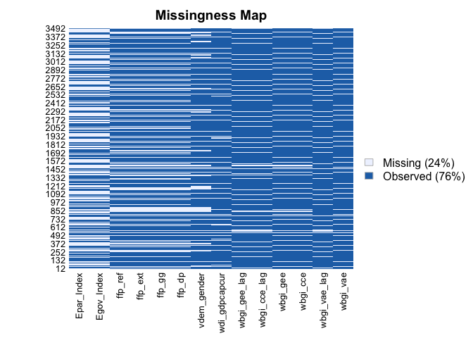
Next is the missing data map of the dataset, which shows that a considerable amount of missing observations are clustered at the EGDI. As discussed before, however, it is due to the fact that the UN E-Government Survey is published once in every two years that caused half of the years in the dataset “missing” the values of the Independent variable rather than the UN being unable to collect data in some of the member states. As for the indicators coming from the Fund for Peace, despite the FSI’s exclusion of 15 UN member states due to the lack of sufficient data sources, it still covers 178 UN member states and thus should not critically compromise the geographical coverage of the statistical analysis. Overall, missing data on observations is unlikely to be a serious issue.
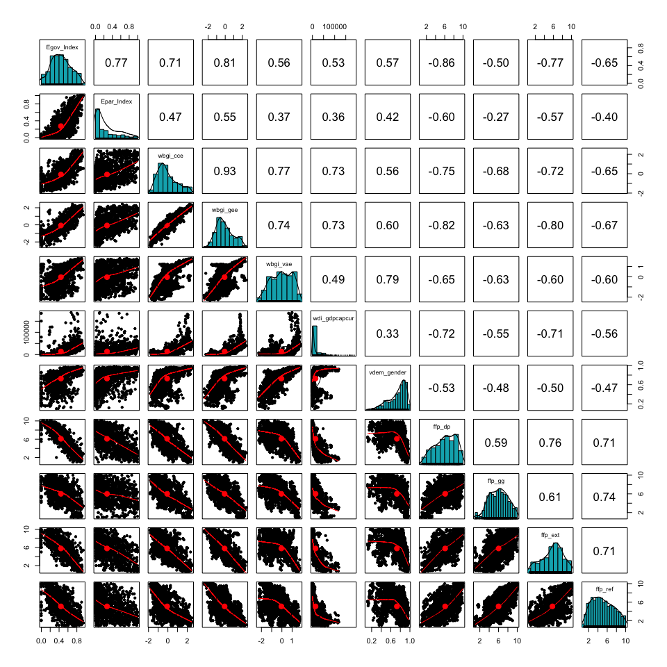
Skewness of variables
Lastly I take a brief look at the skewness of the variables by both numerical measures and the scatter plot matrix. Since the skewness of wdi_gdpcapcur is particularly high among all of the variables (in fact it is the only variable that has a skewness of higher than 1), I will log-transform this variable to prevent it from biasing the regression results.
Skewness in numerical terms
library(moments)
skewness(dataset[c(6, 7, 11:19)], na.rm = T)

##    Egov_Index    Epar_Index      wbgi_cce      wbgi_gee      wbgi_vae
##     0.1049568     0.9737278     0.7002863     0.4166640    -0.1764773
## wdi_gdpcapcur   vdem_gender        ffp_dp        ffp_gg       ffp_ext
##     3.4496094    -0.9606798    -0.3078969    -0.1093040    -0.3408144
##       ffp_ref
##     0.2512283
Scatter plot matrix with histograms
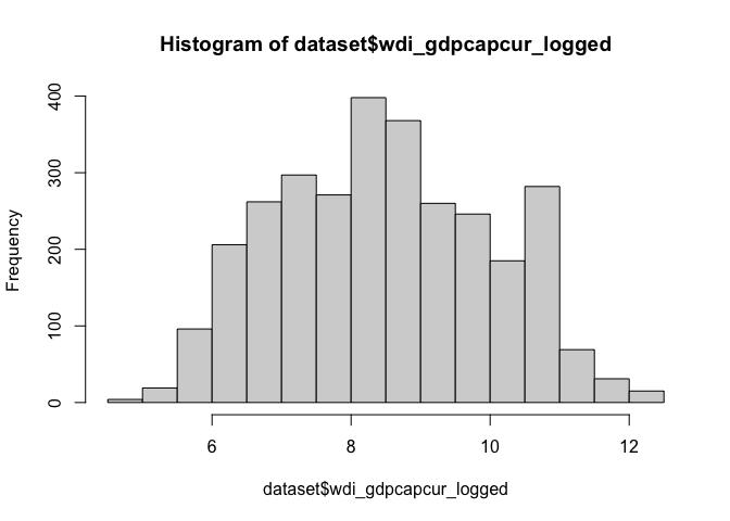
As expected, the wdi_gdpcapcur variable resembles much closer to a normal distribution after being natural log transformed.
dataset = dataset %>%
  mutate(wdi_gdpcapcur_logged = log(wdi_gdpcapcur))
Methodology
Model Selection
Since the data set is panel-structured (i.e. having considerably more units than observations within units across year), it warrants the use of linear mixed effects model since adopting OLS will very likely violate its fundamental assumptions (e.g. assuming the effect of predictors on the response variable and intercept are constant for all observation, no serial correlation among observations). That leaves to the choice between fixed effects and random effects model. Which one should be adopted then?
I will now create models with random effects and fixed effects first before moving on to select which one is the better for each of the dependent variable. For the fixed effects model I will be using the LSDV method, whereas for the random effects model I will add year as the random intercept in one version and country as the random intercept in another. Note that the dummy terms are hidden for the fixed effects specifications to avoid excessively long tables.
Regression tables of random effects and fixed effects models
Dependent Variable: Control of Corruption Indicator (lagged 2 years)
| RE with country as random intercept | RE with year as random intercept | FE with country dummies | |||||||
|---|---|---|---|---|---|---|---|---|---|
| Predictors | Estimates | std. Error | p | Estimates | std. Error | p | Estimates | std. Error | p |
| (Intercept) | -0.830 | 0.215 | <0.001 | -1.796 | 0.321 | <0.001 | |||
| E-Government Development Index | -0.054 | 0.091 | 0.552 | 1.407 | 0.188 | <0.001 | -0.097 | 0.090 | 0.282 |
| Logged GDP Per Capita in Current USD | 0.096 | 0.019 | <0.001 | 0.203 | 0.025 | <0.001 | 0.056 | 0.020 | 0.006 |
| V-DEM Women political empowerment index | 0.120 | 0.127 | 0.342 | 0.912 | 0.123 | <0.001 | -0.020 | 0.133 | 0.880 |
| Demographic Pressure | -0.017 | 0.009 | 0.054 | -0.053 | 0.016 | 0.001 | -0.013 | 0.009 | 0.123 |
| Group Grievance | -0.039 | 0.009 | <0.001 | -0.133 | 0.012 | <0.001 | -0.020 | 0.009 | 0.031 |
| External Intervention | -0.014 | 0.008 | 0.082 | -0.057 | 0.012 | <0.001 | -0.005 | 0.008 | 0.535 |
| Refugees and IDPs | -0.011 | 0.007 | 0.128 | 0.059 | 0.012 | <0.001 | -0.007 | 0.007 | 0.334 |
| region: Americas | 0.222 | 0.168 | 0.186 | -0.485 | 0.054 | <0.001 | -1.328 | 0.234 | <0.001 |
| region: Asia | 0.144 | 0.144 | 0.315 | -0.227 | 0.050 | <0.001 | -1.382 | 0.199 | <0.001 |
| region: Europe | 0.891 | 0.157 | <0.001 | -0.427 | 0.064 | <0.001 | 1.452 | 0.239 | <0.001 |
| region: Oceania | 0.881 | 0.328 | 0.007 | 0.248 | 0.098 | 0.012 | -0.393 | 0.206 | 0.056 |
| region: Africa | -1.291 | 0.209 | <0.001 | ||||||
| Random Effects | |||||||||
| σ2 | 0.03 | 0.25 | |||||||
| τ00 | 0.48 cname | 0.02 year | |||||||
| ICC | 0.95 | 0.06 | |||||||
| N | 169 cname | 7 year | |||||||
| Observations | 1132 | 1132 | 1132 | ||||||
| Marginal R2 / Conditional R2 | 0.397 / 0.969 | 0.745 / 0.761 | 0.979 / 0.975 | ||||||
| AIC | -22.087 | 1743.708 | -759.239 | ||||||
Dependent Variable: Government Effectiveness Indicator (lagged 2 years)
| RE with country as random intercept | RE with year as random intercept | FE with country dummies | |||||||
|---|---|---|---|---|---|---|---|---|---|
| Predictors | Estimates | std. Error | p | Estimates | std. Error | p | Estimates | std. Error | p |
| (Intercept) | -0.472 | 0.201 | 0.019 | -1.912 | 0.251 | <0.001 | |||
| E-Government Development Index | 0.047 | 0.088 | 0.593 | 1.663 | 0.146 | <0.001 | -0.021 | 0.087 | 0.811 |
| Logged GDP Per Capita in Current USD | 0.082 | 0.018 | <0.001 | 0.166 | 0.020 | <0.001 | 0.037 | 0.019 | 0.059 |
| V-DEM Women political empowerment index | 0.228 | 0.120 | 0.057 | 1.097 | 0.095 | <0.001 | 0.013 | 0.128 | 0.922 |
| Demographic Pressure | -0.032 | 0.008 | <0.001 | -0.056 | 0.013 | <0.001 | -0.030 | 0.008 | <0.001 |
| Group Grievance | -0.031 | 0.008 | <0.001 | -0.063 | 0.009 | <0.001 | -0.013 | 0.009 | 0.138 |
| External Intervention | -0.053 | 0.008 | <0.001 | -0.088 | 0.009 | <0.001 | -0.041 | 0.008 | <0.001 |
| Refugees and IDPs | -0.027 | 0.007 | <0.001 | 0.040 | 0.009 | <0.001 | -0.024 | 0.007 | 0.001 |
| region: Americas | 0.225 | 0.134 | 0.094 | -0.409 | 0.042 | <0.001 | -0.818 | 0.226 | <0.001 |
| region: Asia | 0.371 | 0.115 | 0.001 | 0.001 | 0.039 | 0.989 | -0.550 | 0.192 | 0.004 |
| region: Europe | 0.814 | 0.128 | <0.001 | -0.348 | 0.050 | <0.001 | 1.538 | 0.230 | <0.001 |
| region: Oceania | 0.490 | 0.260 | 0.060 | -0.027 | 0.076 | 0.725 | -0.455 | 0.199 | 0.022 |
| region: Africa | -0.630 | 0.202 | 0.002 | ||||||
| Random Effects | |||||||||
| σ2 | 0.02 | 0.15 | |||||||
| τ00 | 0.30 cname | 0.02 year | |||||||
| ICC | 0.92 | 0.11 | |||||||
| N | 169 cname | 7 year | |||||||
| Observations | 1132 | 1132 | 1132 | ||||||
| Marginal R2 / Conditional R2 | 0.573 / 0.967 | 0.830 / 0.849 | 0.979 / 0.975 | ||||||
| AIC | -158.480 | 1170.621 | -838.562 | ||||||
Dependent Variable: Voice and Accountability Indicator (lagged 2 years)
| RE with country as random intercept | RE with year as random intercept | FE with country dummies | |||||||
|---|---|---|---|---|---|---|---|---|---|
| Predictors | Estimates | std. Error | p | Estimates | std. Error | p | Estimates | std. Error | p |
| (Intercept) | -1.433 | 0.208 | <0.001 | -2.976 | 0.306 | <0.001 | |||
| E-Government Development Index | 0.272 | 0.091 | 0.003 | 0.472 | 0.181 | 0.009 | 0.236 | 0.092 | 0.010 |
| Logged GDP Per Capita in Current USD | 0.024 | 0.019 | 0.208 | 0.120 | 0.024 | <0.001 | 0.000 | 0.020 | 0.985 |
| V-DEM Women political empowerment index | 1.282 | 0.124 | <0.001 | 2.704 | 0.120 | <0.001 | 0.977 | 0.135 | <0.001 |
| Demographic Pressure | 0.005 | 0.009 | 0.549 | 0.011 | 0.016 | 0.505 | 0.006 | 0.009 | 0.490 |
| Group Grievance | -0.039 | 0.009 | <0.001 | -0.099 | 0.012 | <0.001 | -0.022 | 0.009 | 0.015 |
| External Intervention | 0.004 | 0.008 | 0.599 | -0.007 | 0.012 | 0.557 | 0.012 | 0.009 | 0.164 |
| Refugees and IDPs | -0.021 | 0.007 | 0.003 | 0.018 | 0.012 | 0.126 | -0.017 | 0.007 | 0.016 |
| region: Americas | 0.490 | 0.136 | <0.001 | 0.125 | 0.053 | 0.019 | -1.535 | 0.238 | <0.001 |
| region: Asia | -0.095 | 0.116 | 0.414 | -0.103 | 0.049 | 0.034 | -1.506 | 0.202 | <0.001 |
| region: Europe | 0.908 | 0.130 | <0.001 | 0.249 | 0.062 | <0.001 | 0.339 | 0.242 | 0.162 |
| region: Oceania | 0.911 | 0.264 | 0.001 | 0.712 | 0.096 | <0.001 | -0.330 | 0.209 | 0.114 |
| region: Africa | -1.935 | 0.212 | <0.001 | ||||||
| Random Effects | |||||||||
| σ2 | 0.03 | 0.24 | |||||||
| τ00 | 0.31 cname | 0.00 year | |||||||
| ICC | 0.92 | 0.01 | |||||||
| N | 169 cname | 7 year | |||||||
| Observations | 1132 | 1132 | 1132 | ||||||
| Marginal R2 / Conditional R2 | 0.593 / 0.967 | 0.747 / 0.748 | 0.977 / 0.972 | ||||||
| AIC | -70.574 | 1685.594 | -728.324 | ||||||
From the above tables, the random effects model with year as the random intercept is the worst-performing one for all the dependent variables because it has the highest AIC value. That leaves the choice between the random effects model with country as the random intercept and the fixed effects model with country dummies. Here I will use the Hausman’s Test to prompt whether the estimation of coefficients between the two models is statistically significantly different:
Hausman’s test result by dependent variable
Dependent Variable: Control of Corruption Indicator (lagged 2 years)
hausman_test(lm_re_CC_cname, lm_fe_CC)

##
##  Hausman Test
##
## data:  dataset
## chisq = 456.54, df = 11, p-value < 2.2e-16
## alternative hypothesis: one model is inconsistent
Dependent Variable: Government Effectiveness Indicator (lagged 2 years)
hausman_test(lm_re_GE_cname, lm_fe_GE)

##
##  Hausman Test
##
## data:  dataset
## chisq = 21.811, df = 11, p-value = 0.02588
## alternative hypothesis: one model is inconsistent
Dependent Variable: Voice and Accountability Indicator (lagged 2 years)
hausman_test(lm_re_VA_cname, lm_fe_VA)

##
##  Hausman Test
##
## data:  dataset
## chisq = 26.017, df = 11, p-value = 0.006451
## alternative hypothesis: one model is inconsistent
The Hausman’s test shows that the difference in the estimation of coefficients between the random effects and fixed effects models are statistically significant at the 95% level for all of the dependent variables. While this can be an evidence to support the use of fixed effects models, I decided to use random effects model with country as the random intercept because some of the predictors (including the main independent variable the EGDI) in the regression are slow-moving within units over time, thus making the use of fixed effects model to discard the influence of these sluggish variables on the dependent variables and bias the results. Moreover, there are also not a really large number of observations per unit, which supports the use of random effects model as Clark and Linzer (2015) suggest. Below is the model that I will choose for diagnosis and interpretation in the subsequent section.
| Control of Corruption (lagged 2 years) | Government Effectiveness (lagged 2 years) | Voice and Accountability (lagged 2 years) | |||||||
|---|---|---|---|---|---|---|---|---|---|
| Predictors | Estimates | std. Error | p | Estimates | std. Error | p | Estimates | std. Error | p |
| (Intercept) | -0.830 | 0.215 | <0.001 | -0.472 | 0.201 | 0.019 | -1.433 | 0.208 | <0.001 |
| E-Government Development Index | -0.054 | 0.091 | 0.552 | 0.047 | 0.088 | 0.593 | 0.272 | 0.091 | 0.003 |
| Logged GDP Per Capita in Current USD | 0.096 | 0.019 | <0.001 | 0.082 | 0.018 | <0.001 | 0.024 | 0.019 | 0.208 |
| V-DEM Women political empowerment index | 0.120 | 0.127 | 0.342 | 0.228 | 0.120 | 0.057 | 1.282 | 0.124 | <0.001 |
| Demographic Pressure | -0.017 | 0.009 | 0.054 | -0.032 | 0.008 | <0.001 | 0.005 | 0.009 | 0.549 |
| Group Grievance | -0.039 | 0.009 | <0.001 | -0.031 | 0.008 | <0.001 | -0.039 | 0.009 | <0.001 |
| External Intervention | -0.014 | 0.008 | 0.082 | -0.053 | 0.008 | <0.001 | 0.004 | 0.008 | 0.599 |
| Refugees and IDPs | -0.011 | 0.007 | 0.128 | -0.027 | 0.007 | <0.001 | -0.021 | 0.007 | 0.003 |
| region: Americas | 0.222 | 0.168 | 0.186 | 0.225 | 0.134 | 0.094 | 0.490 | 0.136 | <0.001 |
| region: Asia | 0.144 | 0.144 | 0.315 | 0.371 | 0.115 | 0.001 | -0.095 | 0.116 | 0.414 |
| region: Europe | 0.891 | 0.157 | <0.001 | 0.814 | 0.128 | <0.001 | 0.908 | 0.130 | <0.001 |
| region: Oceania | 0.881 | 0.328 | 0.007 | 0.490 | 0.260 | 0.060 | 0.911 | 0.264 | 0.001 |
| Random Effects | |||||||||
| σ2 | 0.03 | 0.02 | 0.03 | ||||||
| τ00 | 0.48 cname | 0.30 cname | 0.31 cname | ||||||
| ICC | 0.95 | 0.92 | 0.92 | ||||||
| N | 169 cname | 169 cname | 169 cname | ||||||
| Observations | 1132 | 1132 | 1132 | ||||||
| Marginal R2 / Conditional R2 | 0.397 / 0.969 | 0.573 / 0.967 | 0.593 / 0.967 | ||||||
| AIC | -22.087 | -158.480 | -70.574 | ||||||
Diagnosis
Now I will check whether assumption are violated in the random effects model and, if so, what remedies could be employed before interpreting the regression results. I am following the guidelines of how to diagnose assumptions of linear mixed-effect models by Palmeri (n.d.).
Linearity
For this assumption I will plot the residuals vis-a-vis the observed value of the dependent variables in each model. Ideally the black line should be closed to the red, horizontal line at y = 0 (i.e. linearity between independent and dependent variables is satisfied). As observed from the residual plots, the relationship between the predictors and the dependent variable is largely linear when the Control of Corruption and Government Effectiveness indicators are the dependent variables.
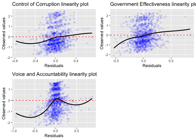
By contrast, the relationship between the predictors and the dependent variable appears to be less linear when the Voice and Accountability indicator is the dependent variable. Therefore, I will add a second-degree term of the EGDI to account for the possibility non-linearity between the predictors and the dependent variable. As shown below, the second-degree term of the EGDI is indeed statistically significant at the 95% level when the Voice and Accountability Indicator is the dependent variable, thereby implying a non-linear relationship between the EGDI and the Voice and Accountability Indicator.
| Voice and Accountability (lagged 2 years) | |||
|---|---|---|---|
| Predictors | Estimates | std. Error | p |
| (Intercept) | -1.400 | 0.208 | <0.001 |
| E-Government Development Index | 0.821 | 0.208 | <0.001 |
| I(Egov\_Index^2) | -0.592 | 0.202 | 0.003 |
| Logged GDP Per Capita in Current USD | 0.016 | 0.019 | 0.388 |
| V-DEM Women political empowerment index | 1.257 | 0.124 | <0.001 |
| Demographic Pressure | -0.001 | 0.009 | 0.896 |
| Group Grievance | -0.037 | 0.009 | <0.001 |
| External Intervention | 0.002 | 0.008 | 0.852 |
| Refugees and IDPs | -0.022 | 0.007 | 0.002 |
| region: Americas | 0.473 | 0.138 | 0.001 |
| region: Asia | -0.113 | 0.118 | 0.338 |
| region: Europe | 0.908 | 0.132 | <0.001 |
| region: Oceania | 0.919 | 0.268 | 0.001 |
| Random Effects | |||
| σ2 | 0.03 | ||
| τ00 cname | 0.32 | ||
| ICC | 0.92 | ||
| N cname | 169 | ||
| Observations | 1132 | ||
| Marginal R2 / Conditional R2 | 0.586 / 0.968 | ||
| AIC | -75.680 | ||
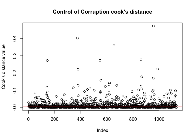
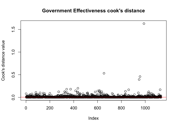
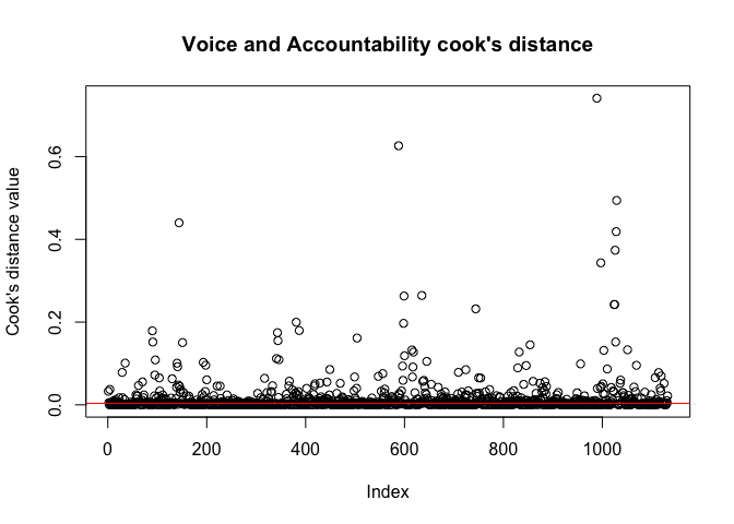
Influential observations
I will use the cook’s distance plot to gauge whether there are influential observations in the model. The threshold of the cook’s distance will be 4/1133 = 0.00353045 to classify which observations are influential in terms of how much impact will be on the model after deleting them from the regression model.
Dependent Variable: Control of Corruption Indicator (lagged 2 years)
## integer(0)
Dependent Variable: Government Effectiveness Indicator (lagged 2 years)
## integer(0)
Dependent Variable: Voice and Accountability Indicator (lagged 2 years)
## integer(0)
The cook’s distance of most observations fall closely the threshold in all three models, but there are a few observations that exert much higher influence on the regression results. However, since this study is observational and these outliers indeed exist and are observed in the real world, removing them may risk ignoring information about how e-governance is associated with governance quality in reality. Furthermore, given there are over 1100 observations in the model, the presence of outliers is unlikely to drastically change the estimated coefficients. Therefore, I decided not to delete these highly influential observations.
Normality of the residuals
I will use the Shapiro-Wilk test to diagnose whether the error term is normally distributed and has an expected value of zero, with the null hypothesis that the error term is normally distributed whilst the alternative hypothesis is that it is not.
Dependent Variable: Control of Corruption Indicator (lagged 2 years)
shapiro.test(diag_CC$.resid)

##
##  Shapiro-Wilk normality test
##
## data:  diag_CC$.resid
## W = 0.98182, p-value = 1.061e-10
Dependent Variable: Government Effectiveness Indicator (lagged 2 years)
shapiro.test(diag_GE$.resid)

##
##  Shapiro-Wilk normality test
##
## data:  diag_GE$.resid
## W = 0.98153, p-value = 8.204e-11
Dependent Variable: Voice and Accountability Indicator (lagged 2 years)
shapiro.test(diag_VA$.resid)

##
##  Shapiro-Wilk normality test
##
## data:  diag_VA$.resid
## W = 0.92162, p-value < 2.2e-16
Here, the p-values are all smaller than 0.05 in the Shapiro-Wilk test for the three models, thereby supporting the alternative hypothesis that the error term is not normally distributed in the models. Nevertheless, since my research question is primarily interested in testing whether e-governance is associated with higher governance quality from 2003-18 (i.e. estimation) instead of using the regression results to generate predictions of how improvement in e-governance may bolster governance quality in the future, violating the assumption of normally distributed residuals is not critical in regard to my research question.
Homoscedasticity
Next I will test probably one of the most important assumptions called homoscedasticity, which means the error term has equal variance. Here I am plotting the fitted values versus the residuals. Ideally the black line should be closed to the red, horizontal line at y = 0 (i.e. the residuals have equal variance).
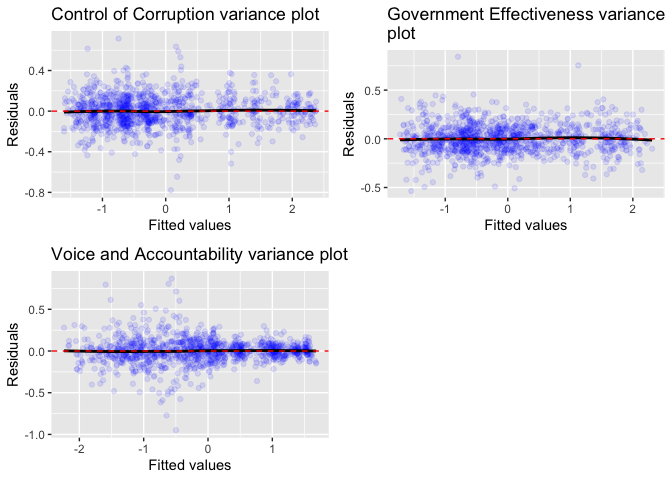
It appears that the black lines closely align to the red line, meaning that the residuals have equal variance across all levels of the explanatory variables. Therefore, the homoscedasticity assumption can be said to be satisfied in the model.
Multi-collinearity
In terms of multicollinearity, I will check whether the predictors have Variance inflation factor (VIF) values which are higher than 4 as the threshold.
Dependent Variable: Control of Corruption Indicator (lagged 2 years)
vif(lm_re_CC_cname)

##                          GVIF Df GVIF^(1/(2*Df))
## Egov_Index           1.470686  1        1.212718
## wdi_gdpcapcur_logged 1.399278  1        1.182911
## vdem_gender          1.159931  1        1.077001
## ffp_dp               1.470419  1        1.212608
## ffp_gg               1.089484  1        1.043783
## ffp_ext              1.256714  1        1.121032
## ffp_ref              1.202997  1        1.096812
## region               1.208657  4        1.023971
Dependent Variable: Government Effectiveness Indicator (lagged 2 years)
vif(lm_re_GE_cname)

##                          GVIF Df GVIF^(1/(2*Df))
## Egov_Index           1.520746  1        1.233185
## wdi_gdpcapcur_logged 1.470558  1        1.212666
## vdem_gender          1.186420  1        1.089229
## ffp_dp               1.520710  1        1.233171
## ffp_gg               1.103482  1        1.050467
## ffp_ext              1.294411  1        1.137722
## ffp_ref              1.231598  1        1.109774
## region               1.292989  4        1.032641
Dependent Variable: Voice and Accountability Indicator (lagged 2 years)
vif(lm_re_VA_cname)

##                          GVIF Df GVIF^(1/(2*Df))
## Egov_Index           8.019378  1        2.831851
## I(Egov_Index^2)      8.149187  1        2.854678
## wdi_gdpcapcur_logged 1.496619  1        1.223364
## vdem_gender          1.189946  1        1.090846
## ffp_dp               1.620748  1        1.273086
## ffp_gg               1.108285  1        1.052751
## ffp_ext              1.317147  1        1.147670
## ffp_ref              1.234163  1        1.110929
## region               1.304067  4        1.033743
Besides the second-degree term of the EGDI being highly collinear with its first-degree counterpart in the model where the Voice and Accountability is the dependent variable (which should not be surprising), all other predictors have their VIF values smaller than 4 in all models. Thus, multicollinearity is very unlikely to be a concern.
Endogeneity
The modelling process has taken the endogeneity issue into account via two ways. Firstly, I have lagged the dependent variables by two years so as to alleviate omitted variable bias. As for autocorrelation, since this is almost certainly the case in panel data setting, this is the reason for why I chose to adopt linear mixed effects model in the first place to account for this issue in addition to lagging the dependent variables by 2 years.
Results
After checking for the model assumptions and performing relevant remedies, I will present the following models for the interpretation:
| Model (1): Control of Corruption (lagged 2 years) | Model (2): Government Effectiveness (lagged 2 years) | Model (3): Voice and Accountability (lagged 2 years) | |||||||
|---|---|---|---|---|---|---|---|---|---|
| Predictors | Estimates | std. Error | p | Estimates | std. Error | p | Estimates | std. Error | p |
| (Intercept) | -0.830 | 0.215 | <0.001 | -0.472 | 0.201 | 0.019 | -1.400 | 0.208 | <0.001 |
| E-Government Development Index | -0.054 | 0.091 | 0.552 | 0.047 | 0.088 | 0.593 | 0.821 | 0.208 | <0.001 |
| Logged GDP Per Capita in Current USD | 0.096 | 0.019 | <0.001 | 0.082 | 0.018 | <0.001 | 0.016 | 0.019 | 0.388 |
| V-DEM Women political empowerment index | 0.120 | 0.127 | 0.342 | 0.228 | 0.120 | 0.057 | 1.257 | 0.124 | <0.001 |
| Demographic Pressure | -0.017 | 0.009 | 0.054 | -0.032 | 0.008 | <0.001 | -0.001 | 0.009 | 0.896 |
| Group Grievance | -0.039 | 0.009 | <0.001 | -0.031 | 0.008 | <0.001 | -0.037 | 0.009 | <0.001 |
| External Intervention | -0.014 | 0.008 | 0.082 | -0.053 | 0.008 | <0.001 | 0.002 | 0.008 | 0.852 |
| Refugees and IDPs | -0.011 | 0.007 | 0.128 | -0.027 | 0.007 | <0.001 | -0.022 | 0.007 | 0.002 |
| region: Americas | 0.222 | 0.168 | 0.186 | 0.225 | 0.134 | 0.094 | 0.473 | 0.138 | 0.001 |
| region: Asia | 0.144 | 0.144 | 0.315 | 0.371 | 0.115 | 0.001 | -0.113 | 0.118 | 0.338 |
| region: Europe | 0.891 | 0.157 | <0.001 | 0.814 | 0.128 | <0.001 | 0.908 | 0.132 | <0.001 |
| region: Oceania | 0.881 | 0.328 | 0.007 | 0.490 | 0.260 | 0.060 | 0.919 | 0.268 | 0.001 |
| I(Egov\_Index^2) | -0.592 | 0.202 | 0.003 | ||||||
| Random Effects | |||||||||
| σ2 | 0.03 | 0.02 | 0.03 | ||||||
| τ00 | 0.48 cname | 0.30 cname | 0.32 cname | ||||||
| ICC | 0.95 | 0.92 | 0.92 | ||||||
| N | 169 cname | 169 cname | 169 cname | ||||||
| Observations | 1132 | 1132 | 1132 | ||||||
| Marginal R2 / Conditional R2 | 0.397 / 0.969 | 0.573 / 0.967 | 0.586 / 0.968 | ||||||
| AIC | -22.087 | -158.480 | -75.680 | ||||||
From the above regression table, there are 1132 observations for each model, and the high Intraclass Correlation Coefficient (ICC) values in each model (> 0.75) supports the decision of using linear mixed effects model in the first place. The random intercept of countries is different for each dependent variable, namely, it is 0.48 when the dependent variable is the Control of Corruption Indicator, 0.3 when the dependent variable is the Government Effectiveness Indicator and 0.32 when the dependent variable is the Voice and Accountability Indicator.
Forest-plots of estimated coefficients
To better visualise the estimated coefficients and their confidence intervals before interpreting the significance of the results, I will be using the forest plots.
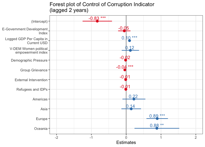
Dependent variable: Control of Corruption Indicator (lagged 2 years)
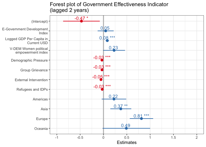
Dependent variable: Government Effectiveness Indicator (lagged 2 years)
Dependent variable: Voice and Accountability Indicator (lagged 2 years)
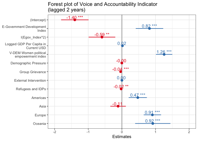
Starting with the significance of the main independent variable, the EGDI score, its coefficients are only statistically significant at the 99% level when the dependent variable is the Voice and Accountability Indicator after adjusting for other factors. To interpret the substantive significance, the marginal effect of one-unit change of the EGDI score is expected to be associated with 0.821 ⋅ EGD**I − 0.592 ⋅ EGD**I2 unit change of the Voice and Accountability Indicator on average after adjusting for other factors. For instance, if the EGDI takes the level of its mean (i.e. 0.441), then it is expected to be associated with 0.821 ⋅ 0.441 − 0.592 ⋅ 0.4412 = 0.247-unit increase of the Voice and Accountability Indicator on average after controlling for other factors. The positive coefficient of the first-degree EGDI term and the negative second-degree EGDI term together suggest that while the marginal effect of Egov_Index on wbgi_vae, after controlling for other variables, starts positive, it will go down and eventually turn negative as the value of Egov_Index becomes larger. By contrast, although the directions of the EGDI’s coefficients are also negative and positive as expected when the dependent variable is respectively the Control of Corruption and the Government Effectiveness Indicators, they are statistically indistinguishable from zero, meaning there is no support for H1 and H2. The result provides mixed evidence for H3, since although initial increase in e-governance is predicted with increase in government’s accountability, once a country’s level of e-governance reaches a certain point, its accountability is actually predicted to start declining after controlling for other factors.
As for the control variables, I will only report those which are statistically significant at least at the 90% level and their directions, ceteris paribus, in this paragraph because they are not the main interest in this research. Starting with economic development level, higher level of economic development is expected to be associated with better control of corruption and public service provision as the coefficients of the logged GDP per capita in current USD are positive and statistically significant at the 99% level in Models (1) and (2). Gender equality is also predicted to be associated with better government effectiveness and more accountability of the government as the coefficients of V-DEM Women political empowerment index are positive and statistically significant at least at the 90% level in Models (2) and (3). Higher demographic pressure may also strain a government’s ability to control corruption and provide adequate public service as shown by the negative coefficients in Models (1) and (2). Likewise, higher hostility among socio-political groups is expected to be associated with worse government performance in controlling corruption, providing public services and accountability to citizens as evidenced by the negative and statistically significant coefficients of Group Grievance in all models. As a country’s governance is intervened to a larger extent by foreign actors, the country may be less capable of mitigating corruption and providing public services effectively as demonstrated by the negative coefficients of External Intervention in models (1) and (2). Higher pressure from displaced population within a country may also reduce the capacity of a government to provide public services and its accountability, as the coefficients of Refugees and IDPs are negative in models (2) and (3).
As for different regions in the world, relative to Africa after adjusting for other factors, Europe and Oceania have better control over corruption, all other regions are more effective in providing public services, and governments in all regions except Asia are more accountable. All of these regional differences in governance quality are statistically significant at least at the 90% level as shown in the regression table.
Robustness Check
Besides checking whether the assumptions are satisfied in previous section, I will now perform some additional robustness check on the model. I will rerun the models with alternative measures as the dependent variables. For model (1), I will use the Bayesian Corruption Indicator (bci_bci) which ranges from 0 to 100 and a higher value indicates that corruption is worse in a country (Teorell et al. 2021) (note that the latest value available of this measure is in 2017). For model (2), I will use the FSI Public Services indicator (ffp_ps) which ranges from 0 to 10 and higher values means worse performance in this regard. For model (3), I will use the Freedom House’s score (FH_Total) which ranges from 0 to 100 and a higher value means a country is more democratic (and thus more accountable). The below correlation test shows that these measures are suitable for being alternative dependent variables since they are strongly correlated with their respective World Bank Indicators counterparts, which can be evidence that they are measuring similar aspects of governance quality. Moreover, these alternative dependent variables are lagged two years as well.
Correlation test of the alternative dependent variables
WGI Control of Corruption Indicator and Bayesian Corruption Indicator
cor.test(dataset$wbgi_cce, dataset$bci_bci)

##
##  Pearson's product-moment correlation
##
## data:  dataset$wbgi_cce and dataset$bci_bci
## t = -120.77, df = 2840, p-value < 2.2e-16
## alternative hypothesis: true correlation is not equal to 0
## 95 percent confidence interval:
##  -0.9206838 -0.9086851
## sample estimates:
##        cor
## -0.9148862
WGI Government Effectiveness Indicator and FSI Public Services Indicator
cor.test(dataset$wbgi_gee, dataset$ffp_ps)

##
##  Pearson's product-moment correlation
##
## data:  dataset$wbgi_gee and dataset$ffp_ps
## t = -92.625, df = 2438, p-value < 2.2e-16
## alternative hypothesis: true correlation is not equal to 0
## 95 percent confidence interval:
##  -0.8909305 -0.8733467
## sample estimates:
##        cor
## -0.8824465
WGI Voice and Accountability Indicator and Freedom House Regime Score
cor.test(dataset$wbgi_vae, dataset$FH_Total)

##
##  Pearson's product-moment correlation
##
## data:  dataset$wbgi_vae and dataset$FH_Total
## t = 224.74, df = 2794, p-value < 2.2e-16
## alternative hypothesis: true correlation is not equal to 0
## 95 percent confidence interval:
##  0.9714230 0.9753142
## sample estimates:
##       cor
## 0.9734388
dataset = dataset %>%
  mutate(FH_Total_lag = Lag(FH_Total, 2)) %>%
  mutate(bci_bci_lag = Lag(bci_bci, 2)) %>%
  mutate(ffp_ps_lag = Lag(ffp_ps, 2))
Regression results of alternative dependent variables
Model (1) for testing H1
| WGI Control of corruption | Bayesian Corruption Indicator | |||||
|---|---|---|---|---|---|---|
| Predictors | Estimates | std. Error | p | Estimates | std. Error | p |
| (Intercept) | -0.830 | 0.215 | <0.001 | 63.156 | 3.242 | <0.001 |
| E-Government Development Index | -0.054 | 0.091 | 0.552 | -4.098 | 1.303 | 0.002 |
| Logged GDP Per Capita in Current USD | 0.096 | 0.019 | <0.001 | -1.655 | 0.280 | <0.001 |
| V-DEM Women political empowerment index | 0.120 | 0.127 | 0.342 | 2.163 | 1.849 | 0.242 |
| Demographic Pressure | -0.017 | 0.009 | 0.054 | -0.025 | 0.124 | 0.841 |
| Group Grievance | -0.039 | 0.009 | <0.001 | 0.192 | 0.127 | 0.130 |
| External Intervention | -0.014 | 0.008 | 0.082 | 0.363 | 0.120 | 0.002 |
| Refugees and IDPs | -0.011 | 0.007 | 0.128 | 0.109 | 0.102 | 0.285 |
| region: Americas | 0.222 | 0.168 | 0.186 | 0.987 | 2.911 | 0.735 |
| region: Asia | 0.144 | 0.144 | 0.315 | -4.562 | 2.494 | 0.067 |
| region: Europe | 0.891 | 0.157 | <0.001 | -11.277 | 2.692 | <0.001 |
| region: Oceania | 0.881 | 0.328 | 0.007 | -15.947 | 5.706 | 0.005 |
| Random Effects | ||||||
| σ2 | 0.03 | 5.43 | ||||
| τ00 | 0.48 cname | 146.64 cname | ||||
| ICC | 0.95 | 0.96 | ||||
| N | 169 cname | 169 cname | ||||
| Observations | 1132 | 1132 | ||||
| Marginal R2 / Conditional R2 | 0.397 / 0.969 | 0.300 / 0.975 | ||||
| AIC | -22.087 | 6007.555 | ||||
Model (2) for testing H2
| WGI Government Effectiveness | FSI Public Services | |||||
|---|---|---|---|---|---|---|
| Predictors | Estimates | std. Error | p | Estimates | std. Error | p |
| (Intercept) | -0.472 | 0.201 | 0.019 | 7.152 | 0.661 | <0.001 |
| E-Government Development Index | 0.047 | 0.088 | 0.593 | -0.604 | 0.277 | 0.029 |
| Logged GDP Per Capita in Current USD | 0.082 | 0.018 | <0.001 | -0.473 | 0.054 | <0.001 |
| V-DEM Women political empowerment index | 0.228 | 0.120 | 0.057 | 0.089 | 0.278 | 0.750 |
| Demographic Pressure | -0.032 | 0.008 | <0.001 | 0.361 | 0.028 | <0.001 |
| Group Grievance | -0.031 | 0.008 | <0.001 | 0.052 | 0.023 | 0.024 |
| External Intervention | -0.053 | 0.008 | <0.001 | 0.096 | 0.023 | <0.001 |
| Refugees and IDPs | -0.027 | 0.007 | <0.001 | 0.050 | 0.022 | 0.021 |
| region: Americas | 0.225 | 0.134 | 0.094 | -0.219 | 0.173 | 0.206 |
| region: Asia | 0.371 | 0.115 | 0.001 | -0.747 | 0.148 | <0.001 |
| region: Europe | 0.814 | 0.128 | <0.001 | -0.998 | 0.187 | <0.001 |
| region: Oceania | 0.490 | 0.260 | 0.060 | -0.385 | 0.318 | 0.226 |
| Random Effects | ||||||
| σ2 | 0.02 | 0.20 | ||||
| τ00 | 0.30 cname | 0.40 cname | ||||
| ICC | 0.92 | 0.67 | ||||
| N | 169 cname | 168 cname | ||||
| Observations | 1132 | 990 | ||||
| Marginal R2 / Conditional R2 | 0.573 / 0.967 | 0.892 / 0.964 | ||||
| AIC | -158.480 | 1677.371 | ||||
Model (3) for testing H3
| WGI Voice and Accountability | Freedom House Regime Score | |||||
|---|---|---|---|---|---|---|
| Predictors | Estimates | std. Error | p | Estimates | std. Error | p |
| (Intercept) | -1.400 | 0.208 | <0.001 | 15.172 | 7.270 | 0.037 |
| E-Government Development Index | 0.821 | 0.208 | <0.001 | 22.486 | 7.296 | 0.002 |
| I(Egov\_Index^2) | -0.592 | 0.202 | 0.003 | -17.802 | 7.086 | 0.012 |
| Logged GDP Per Capita in Current USD | 0.016 | 0.019 | 0.388 | 1.271 | 0.657 | 0.053 |
| V-DEM Women political empowerment index | 1.257 | 0.124 | <0.001 | 29.496 | 4.288 | <0.001 |
| Demographic Pressure | -0.001 | 0.009 | 0.896 | 0.544 | 0.309 | 0.079 |
| Group Grievance | -0.037 | 0.009 | <0.001 | -0.791 | 0.304 | 0.009 |
| External Intervention | 0.002 | 0.008 | 0.852 | 0.166 | 0.286 | 0.563 |
| Refugees and IDPs | -0.022 | 0.007 | 0.002 | -0.162 | 0.246 | 0.511 |
| region: Americas | 0.473 | 0.138 | 0.001 | 15.598 | 4.355 | <0.001 |
| region: Asia | -0.113 | 0.118 | 0.338 | -9.987 | 3.859 | 0.010 |
| region: Europe | 0.908 | 0.132 | <0.001 | 25.849 | 4.259 | <0.001 |
| region: Oceania | 0.919 | 0.268 | 0.001 | 21.641 | 8.288 | 0.009 |
| Random Effects | ||||||
| σ2 | 0.03 | 30.49 | ||||
| τ00 | 0.32 cname | 298.55 cname | ||||
| ICC | 0.92 | 0.91 | ||||
| N | 169 cname | 156 cname | ||||
| Observations | 1132 | 1048 | ||||
| Marginal R2 / Conditional R2 | 0.586 / 0.968 | 0.529 / 0.956 | ||||
| AIC | -75.680 | 7191.480 | ||||
Regarding the main independent variable (level of e-governance), after using alternative measures for the dependent variables, in Model (1) increase in level of e-governance is statistically significantly associated with better control of corruption when the Bayesian Corruption Indicator is used as the dependent variable since the coefficient of Egov_Index is negative and has a p-value lower than 0.05. Likewise, when the FSI Public Services Indicator is used as the dependent variable in Model (2), the coefficient of the Egov_Index is also negative and statistically significant at the 95% level, again implying more advanced e-governance is associated with better public service provision. However, I am cautious to take these results as evidence supporting H1 and H2, since this can also mean that the results are sensitive to the choice of which measure as the dependent variables. Further investigation is warranted.
As for H3, both the first- and second-degree term of the EGDI are statistically significant at the 95% level and point to the same directions as when the World Bank’s Voice and Accountability Indicator is used as the dependent variable. It seems therefore that H3 still has support even when alternative measure of government accountability is used.
Conclusion
To conclude, I used linear random effects model to investigate the relationship between e-governance level and governance quality in regard to controlling corruption, providing public services and government accountability across UN member states from 2003-18. The regression result suggests that there is a lack of evidence to conclude that more advanced e-governance is associated with less corruption and better public service provision. As for improvement in government accountability, the result offers mixed support because there seems to be a non-linear relationship, namely, although initial advancement in e-governance is associated with more accountable government, once advancement reaches a certain point, the relationship may start to reverse.
In terms of generalisability, since the data set covers most of the UN member states which constitute a large part of the nation-states in the world, cross-section-wise the result should be generalisable. In temporal dimension, however, because of the lack of adequate imputation techniques, half of the years in the data set do not the values of the EGDI. Consequently, not only the number of observations was greatly reduced in the regression analysis, but the argument on whether countries which saw improvement in e-governance level also witness increase in governance quality over the period from 2003 to 2018 could also have been strengthened if imputation techniques had been deployed to fill in the blank years of the main independent variable.
To situate this analysis in the literature, it appears that the relationship between e-governance level and governance quality may not be as straightforward as policy makers and some scholars envision. Putting aside the lack of support towards reducing corruption and enhancing public service quality, even when the regression provides evidence of initial advancement of e-governance to be associated with more government accountability, at higher levels of e-governance the associate may start to turn negative instead. Further investigation of the potential reason for this phenomenon is warranted, which can be started by disaggregating countries according to different categories besides regions such as income level and regime type. Moreover, it may also be important to see whether the improvement of governance quality associated with e-governance is conditional on other factors in the future, because a lot of controls are demonstrated to be significant in associating with governance quality in the regression model.
Of course, this analysis suffers from a few limitations. For starters, this study only investigated the association between advancement in e-governance and some of the many aspects of governance quality. Further studies should explore whether e-governance level may also be associated other aspects of governance quality, and if so, to what direction and how much in substantive terms. Moreover, the EGDI primarily focuses on e-governance initiatives carried out by national government, but undoubtedly non-state actors also play a crucial role in the development of e-governance (e.g. social media platforms are owned by private companies and yet they are an invaluable platform for governments and politicians to publicise information apart from the official websites). Indices that capture e-governance performance in the future should therefore also include the private sector’s contribution of promoting e-governance.
Reference
Bibliography
Bannister, Frank, and Regina Connolly. “Defining e-governance.” e-Service Journal: A Journal of Electronic Services in the Public and Private Sectors 8.2 (2012): 3-25.
Barthwal, C.P. “E-GOVERNANCE FOR GOOD GOVERNANCE.” The Indian Journal of Political Science, vol. 64, no. 3/4, 2003, pp. 285–308. JSTOR, www.jstor.org/stable/41855786. Accessed 1 June 2021.
Clark, Tom S., and Drew A. Linzer. “Should I use fixed or random effects.” Political science research and methods 3.2 (2015): 399-408.
“E-government.” UN E-Government Survey. United Nations, 2021. Web. 31 May 2021. https://publicadministration.un.org/egovkb/en-us/About/UNeGovDD-Framework.
Future of E-Government, Agenda 2020. Paris: OECD, 2008. https://www.oecd.org/governance/eleaders/43340370.pdf
“Information and Communication Technologies (ICT).” UNESCO UIS. 31 May 2021. Web. 31 May 2021. http://uis.unesco.org/en/glossary-term/information-and-communication-technologies-ict
Kaufmann, Daniel, Aart Kraay, and Massimo Mastruzzi. “The Worldwide Governance Indicators: Methodology and Analytical Issues1.” Hague journal on the rule of law 3.2 (2011): 220-246.
Madon, Shirin. “e-Governance for Development.” e-Governance for Development. Palgrave Macmillan, London, 2009. 53-70.
“Methodology.” Fragile States Index. The Fund for Peace, 2018. Web. 01 June 2021. https://fragilestatesindex.org/methodology/.
Mira, Rachid, and Ahmed Hammadache. “Good governance and economic growth: A contribution to the institutional debate about state failure in Middle East and North Africa.” Asian Journal of Middle Eastern and Islamic Studies 11.3 (2017): 107-120.
Palmeri, Michael. “Chapter 18: Testing the Assumptions of Multilevel Models.” A Language, Not a Letter: Learning Statistics in R. n.d. Web. 01 June 2021. https://ademos.people.uic.edu/Chapter18.html#1_preface.
Singh, Gurmeet, R.D. Pathak, Rafia Naz, and Rakesh Belwal. “E‐governance for Improved Public Sector Service Delivery in India, Ethiopia and Fiji.” International Journal of Public Sector Management 23.3 (2010): 254-75. Print.
Smith, Robert Frederick Ingram, and Julian Teicher. “Improving governance and services: can e-government help?.” Chinese Public Administration Review 3.3/4 (2016): 62-70.
Teorell, Jan, Aksel Sundström, Sören Holmberg, Bo Rothstein, Natalia Alvarado Pachon & Cem Mert Dalli. 2021. The Quality of Government Standard Dataset, version Jan21. University of Gothenburg: The Quality of Government Institute, http://www.qog.pol.gu.se doi:10.18157/qogstdjan21
“UN E-Government Survey 2018.” UN E-Government Survey. United Nations, 2018. Web. 01 June 2021. https://publicadministration.un.org/egovkb/en-us/Reports/UN-E-Government-Survey-2018.
R packages
Bates D, Mächler M, Bolker B, Walker S (2015). “Fitting Linear Mixed-Effects Models Using lme4.” Journal of Statistical Software, 67(1), 1–48. doi: 10.18637/jss.v067.i01.
Bolker, Ben et al. (2020). broom.mixed: Tidying Methods for Mixed Models. R package version 0.2.6, https://cran.r-project.org/web/packages/broom.mixed/index.html.
Fox J, Weisberg S (2019). An R Companion to Applied Regression, Third edition. Sage, Thousand Oaks CA. https://socialsciences.mcmaster.ca/jfox/Books/Companion/.
Frank E Harrell Jr (2021). Hmisc: Harrell Miscellaneous. R package version 4.5-0, https://cran.r-project.org/web/packages/Hmisc/index.html.
Honaker J, King G, Blackwell M (2011). “Amelia II: A Program for Missing Data.” Journal of Statistical Software, 45(7), 1–47. https://www.jstatsoft.org/v45/i07/.
Kassambara, Alboukadel (2020). ggpubr: ‘ggplot2’ Based Publication Ready Plots. R package version 0.4.0, https://cran.r-project.org/web/packages/ggpubr/index.html.
Komsta, Lukasz & Frederick Novomestky (2015). moments: Moments, cumulants, skewness, kurtosis and related tests. R package version 0.14, https://cran.r-project.org/web/packages/moments/index.html.
Larmarange, Joseph et al. (2021). labelled: Manipulating Labelled Data. R package version 2.8.0, https://cran.r-project.org/web/packages/labelled/index.html.
Lüdecke D (2021). sjPlot: Data Visualization for Statistics in Social Science. R package version 2.8.8, https://CRAN.R-project.org/package=sjPlot.
Revelle W (2021). psych: Procedures for Psychological, Psychometric, and Personality Research. Northwestern University, Evanston, Illinois. R package version 2.1.3, https://CRAN.R-project.org/package=psych.
Rich, Benjamin (2021). table1: Tables of Descriptive Statistics in HTML. R package version 1.4.1, https://cran.rstudio.com/web/packages/table1/.
Wickham H, Averick M, Bryan J, Chang W, McGowan LD, François R, Grolemund G, Hayes A, Henry L, Hester J, Kuhn M, Pedersen TL, Miller E, Bache SM, Müller K, Ooms J, Robinson D, Seidel DP, Spinu V, Takahashi K, Vaughan D, Wilke C, Woo K, Yutani H (2019). “Welcome to the tidyverse.” Journal of Open Source Software, 4(43), 1686. doi: 10.21105/joss.01686.
Wickham, Hadley et al. (2019). readxl: Read Excel Files. R package version 1.3.1, https://cran.r-project.org/web/packages/readxl/index.html.
Zeileis A, Hothorn T (2002). “Diagnostic Checking in Regression Relationships.” R News, 2(3), 7–10. https://CRAN.R-project.org/doc/Rnews/.
[1] Although there are some scholars who argue for the distinction between the terms e-governance and e-government (e.g. Bannister and Connolly 2012), for the sake of simplicity I will use the two terms interchangeably in this article.
Co-Director
Global Governance Centre
Professor
International Relations and Political Science
President
Global Governance Research Centre Consortium
International institutions and political networks.