Thomas Gmuer
1. Introduction
In his seminal 1951 essay entitled “Building Dwelling Thinking,” Martin Heidegger stressed the co-constitutiveness of building and dwelling, the latter extending well beyond the mere residing in end products of constructions to encompass the whole of Being. (Heidegger, 1971) Inspired by this observation, the present research connects strictly defined housing with the broader environment in which we live to initiate a study of the evolution of living conditions in Switzerland. A growing body of literature in comparative political science, and in particular in the domain of political ecology, focuses on the “livability” of cities around the world. Most of the indexes imagined to measure this livability include a measure of land use in some form. For this research project, I focus on the evolution of land use specifically in Swiss Cantons and cities since the 2012 initiative and 2013 referendum, when the population voted to reduce urban sprawl and to limit the proportion of secondary housing in each municipality of the country.
I wish to check, first, whether the aforementioned political decisions are beginning to achieve their purpose, specifically by examining how livability in Swiss cities has evolved since 2013. A first hypothesis I wish to test is whether Switzerland witnesses a shrinking of wooded and recreational areas in cities, as an unintended consequence of the limitation imposed on sprawling, that is, the extension of the built area in less dense regions. Secondly, I examine whether, with regards to land use, a so-called “Roestigraben” opens up between the Northern German-speaking part of the country and the Latin South, a split often observed and commented upon in political debates about cultural differences within the country. Finally, I test whether housing per se is impacted in the main urban centers, that is, not only if the built area is further concentrated but also if accommodations shrink or become more saturated.
2. Data
I will be using the Confederation’s “standard classification” model, the so-called “NOAS04”, which includes basic categories of land cover and use, and allows for extensive synchronic comparison from the 1979/85 period onward. As of December 2019, almost all of the new data for the “Swiss Land Use Statistics” has been collected for the 2013/2018 period. (23 out of 26 cantons, 3 still missing full coverage) The dataset already contains a restriction of previous surveys to fit the existing data as of December 2019. The data is constructed through an analysis of satellite images collected throughout the relevant periods, whereby the nature and function of the ground coverage is identified.
My main response variable will be the surface of wooded and recreational area per capita, the same indicator used to measure “quality of the environment” in the “Quality of Life” survey for cities and urban centers. (Agglo, 2012). It is numerical, continuous, ratio data. The primary unit of analysis is the 156 “statistical cities” of Switzerland, with 23 Cantons as a secondary level.
My control variables will be the evolution of the population of each municipality across the entire period (numerical, continuous, ratio data), language (dummy, German coded as 1 vs non-German, including bilingual Cantons as 0) as well as a detailed account of empty housing (numerical, discrete data) and housing surface per person (numerical, continuous, ratio data) for 2011-2018 in the 8 largest urban centers, to connect the environmental part of “livability” with the quality of housing in the main cities, that is, the “housing” part of our broader dwelling concept, and of the Swiss “Quality of Life” survey.
All the original data can be accessed on the Swiss Federal Statistical Office Webpage. From the various available datasets, I created a new data frame which compiled all the columns of interest into a single file that I called “Livability”. Combining these measures into a single data frame creates a panel data with variables for 156 cities (23 Cantons) over 4 periods (1979/85, 1992/97, 2004/09 and 2013/18). Time is hence used as numerical, discrete data.
Data Visualization
r = getOption("repos")
r["CRAN"] = "http://cran.us.r-project.org"
options(repos = r)
library(haven)
library(readxl)
Livability <- read_excel("Livability.xlsx")
Livability$language=as_factor(Livability$language)
library(ggplot2)
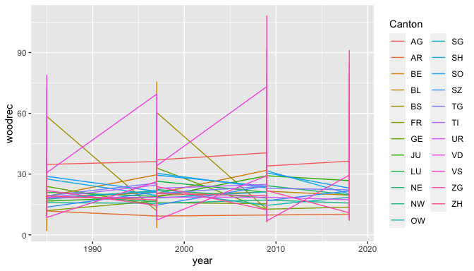
ggplot(data=Livability, aes(x=year, y=woodrec, color= Canton)) + geom_line()
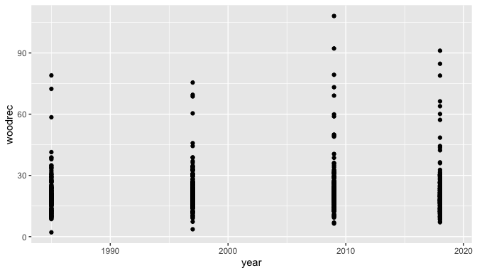
model1 <- ggplot(Livability, aes(year, woodrec))
model1 + geom_point(aes(group = Canton))
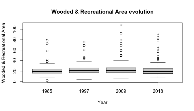
by(Livability$woodrec, Livability$year, summary)

## Livability$year: 1985
##    Min. 1st Qu.  Median    Mean 3rd Qu.    Max.
##    2.10   15.90   19.50   20.97   23.82   79.00
## ------------------------------------------------------------
## Livability$year: 1997
##    Min. 1st Qu.  Median    Mean 3rd Qu.    Max.
##    3.60   17.00   21.10   22.81   26.30   75.50
## ------------------------------------------------------------
## Livability$year: 2009
##    Min. 1st Qu.  Median    Mean 3rd Qu.    Max.
##    6.40   17.05   21.35   24.21   26.43  108.10
## ------------------------------------------------------------
## Livability$year: 2014
##    Min. 1st Qu.  Median    Mean 3rd Qu.    Max.    NA's
##      NA      NA      NA     NaN      NA      NA       8
## ------------------------------------------------------------
## Livability$year: 2015
##    Min. 1st Qu.  Median    Mean 3rd Qu.    Max.    NA's
##      NA      NA      NA     NaN      NA      NA       8
## ------------------------------------------------------------
## Livability$year: 2016
##    Min. 1st Qu.  Median    Mean 3rd Qu.    Max.    NA's
##      NA      NA      NA     NaN      NA      NA       8
## ------------------------------------------------------------
## Livability$year: 2017
##    Min. 1st Qu.  Median    Mean 3rd Qu.    Max.    NA's
##      NA      NA      NA     NaN      NA      NA       8
## ------------------------------------------------------------
## Livability$year: 2018
##    Min. 1st Qu.  Median    Mean 3rd Qu.    Max.    NA's
##   7.043  15.275  19.600  22.357  24.721  91.100       8
## ------------------------------------------------------------
## Livability$year: 2019
##    Min. 1st Qu.  Median    Mean 3rd Qu.    Max.    NA's
##      NA      NA      NA     NaN      NA      NA       8

boxplot(woodrec~year,data=Livability, main="Wooded & Recreational Area evolution",
   xlab="Year", ylab="Wooded & Recreational Area")
3. Methods
I will be using a mixed effects model, with a random effect for Cantons and fixed effects for population, time and language. This modeling choice seems appropriate because we are likely to observe noise caused by canton-correlation in the errors, considering both the wide geographical and sociological differences across Switzerland and the political institutionalization at the Cantonal level that might introduce random Canton-specific trends. Moreover, Cantons capture, in clustering them, part of city-trends as well, albeit in a more manageable way (N= 23 instead of 156)) At the same time, the initial data description shows that there is relatively little variability within Cantons across the 4 periods, thus we also look for fixed effects in time-constant language, and time-varying population. Pooling all panel data in an OLS model would be ill-advised since we violate the assumption that the parameters are the same for all cities/time periods. In the end, we will likely observe variability at the cantonal level that cannot be accounted for completely with our predictors, thus the need for a mixed effects model.
My assumptions are that variations across Cantons are random in the sense that they are not correlated with wooded and recreational area or with other variables of interest. Neither do we expect any major co-correlation across cantons, except for the language one, accounted for as a fixed effect.
4. Results
library("sjPlot")
## Learn more about sjPlot with 'browseVignettes("sjPlot")'.
library(lme4)
## Loading required package: Matrix
re1 <- lmer(woodrec ~ year + (1|Canton), Livability)
re2 <- lmer(woodrec ~ year + log(pop) + (1|Canton), Livability)
re3 <- lmer(woodrec ~ year + language + (1|Canton), Livability)
re4 <- lmer(woodrec ~ year + language + log(pop) + (1|Canton), Livability)
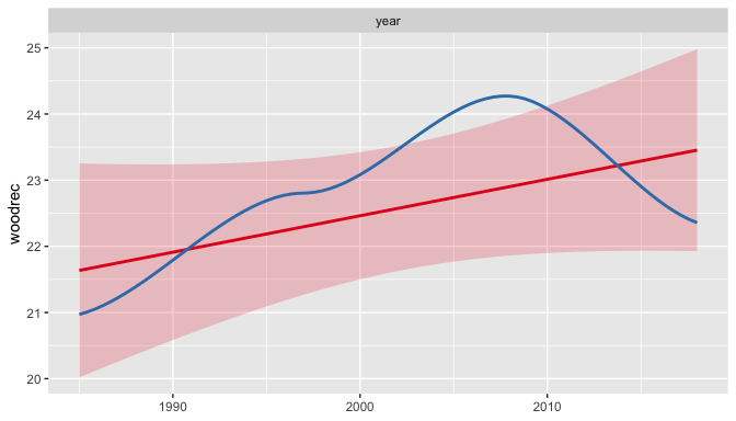
plot_model(re1)
## `geom_smooth()` using formula 'y ~ x'
## `geom_smooth()` using formula 'y ~ x'
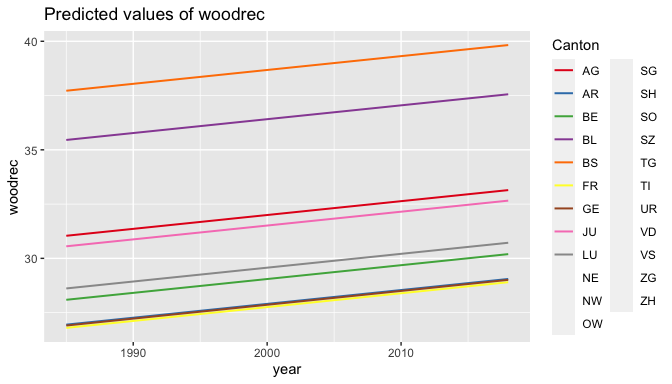
plot_model(re4,  type = "pred", terms = c("year", "Canton"), pred.type="re")

## Model has log-transformed predictors. Consider using `terms="pop [exp]"` to back-transform scale.
tab_model(re1, re2, re3, re4, dv.labels = c("1","2","3","4"), digits = 3, show.aic = T)
| 1 | 2 | 3 | 4 | |||||||||
|---|---|---|---|---|---|---|---|---|---|---|---|---|
| Predictors | Estimates | CI | p | Estimates | CI | p | Estimates | CI | p | Estimates | CI | p |
| (Intercept) | -87.640 | -233.889 – 58.609 | 0.240 | -93.412 | -239.525 – 52.700 | 0.210 | -87.407 | -233.672 – 58.858 | 0.241 | -93.181 | -239.296 – 52.935 | 0.211 |
| year | 0.055 | -0.018 – 0.128 | 0.139 | 0.064 | -0.010 – 0.137 | 0.090 | 0.055 | -0.018 – 0.128 | 0.139 | 0.064 | -0.010 – 0.137 | 0.089 |
| pop \[log\] | -1.191 | -2.568 – 0.187 | 0.090 | -1.200 | -2.580 – 0.179 | 0.088 | ||||||
| language \[1\] | -0.359 | -4.541 – 3.824 | 0.866 | -0.429 | -4.679 – 3.821 | 0.843 | ||||||
| Random Effects | ||||||||||||
| σ2 | 134.04 | 133.51 | 134.01 | 133.46 | ||||||||
| τ00 | 12.88 Canton | 13.43 Canton | 14.00 Canton | 14.67 Canton | ||||||||
| ICC | 0.09 | 0.09 | 0.09 | 0.10 | ||||||||
| N | 23 Canton | 23 Canton | 23 Canton | 23 Canton | ||||||||
| Observations | 624 | 624 | 624 | 624 | ||||||||
| Marginal R2 / Conditional R2 | 0.003 / 0.091 | 0.008 / 0.098 | 0.003 / 0.098 | 0.008 / 0.106 | ||||||||
| AIC | 4861.013 | 4859.021 | 4859.658 | 4857.626 | ||||||||
##
## Attaching package: 'dplyr'

## The following objects are masked from 'package:stats':
##
##     filter, lag

## The following objects are masked from 'package:base':
##
##     intersect, setdiff, setequal, union

filtered <- Livability[which(Livability$year<2010),]
re8 <- lmer(filtered$woodrec ~ filtered$year+filtered$language+log(filtered$pop)+(1|filtered$Canton), Livability)

tab_model(re4, re8, dv.labels = c("4","8"), digits = 3, show.aic = T)
| 4 | 8 | |||||
|---|---|---|---|---|---|---|
| Predictors | Estimates | CI | p | Estimates | CI | p |
| (Intercept) | -93.181 | -239.296 – 52.935 | 0.211 | -249.120 | -455.598 – -42.641 | 0.018 |
| year | 0.064 | -0.010 – 0.137 | 0.089 | |||
| language \[1\] | -0.429 | -4.679 – 3.821 | 0.843 | |||
| pop \[log\] | -1.200 | -2.580 – 0.179 | 0.088 | |||
| filtered$year</td> <td style=" padding:0.2cm; text-align:left; vertical-align:top; text-align:center; "></td> <td style=" padding:0.2cm; text-align:left; vertical-align:top; text-align:center; "></td> <td style=" padding:0.2cm; text-align:left; vertical-align:top; text-align:center; "></td> <td style=" padding:0.2cm; text-align:left; vertical-align:top; text-align:center; ">0.141</td> <td style=" padding:0.2cm; text-align:left; vertical-align:top; text-align:center; ">0.037 – 0.245</td> <td style=" padding:0.2cm; text-align:left; vertical-align:top; text-align:center; col7"><strong>0.008</strong></td> </tr> <tr> <td style=" padding:0.2cm; text-align:left; vertical-align:top; text-align:left; ">filtered$language \[filtered$language1\] | -0.416 | -4.476 – 3.644 | 0.841 | |||
| filtered$pop \[log\] | -1.000 | -2.512 – 0.511 | 0.195 | |||
| Random Effects | ||||||
| σ2 | 133.46 | 124.96 | ||||
| τ00 | 14.67 Canton | 11.41 filtered$Canton | ||||
| ICC | 0.10 | 0.08 | ||||
| N | 23 Canton | 23 filtered$Canton | ||||
| Observations | 624 | 468 | ||||
| Marginal R2 / Conditional R2 | 0.008 / 0.106 | 0.016 / 0.099 | ||||
| AIC | 4857.626 | 3613.679 | ||||
The p values of none of the 3 predictors allow us to reject the null that they have no effect at conventional confidence levels (alpha = 0.05). But considering the non-linear nature of the temporal evolution we expected following our hypothesized mechanism and the trend observed for 2018 in the mean of wooded and recreation area per capita as well as in the basic prediction plot of model 1, it is likely that removing the last period would reinforce this marginal effect of time. After filtering accordingly, time indeed becomes statistically significant (p=0.008), with an increase in wooded and recreational area per capita of 0.141 square meter per year. Language seems far from being statistically significant under any of the two models (p = 0.84), thus disproving the presence of a so-called “Roestigraben” with regards to wooded and recreational area. The (negative) effect of population was close to being statistically significant in model 4, but not in model 8. We then turn to a brief analysis of housing.
re5 <- lmer(surface ~ year + (1|City), Livability)
re6 <- lmer(empty ~ year + (1|City), Livability)
re7 <- lmer(log(overcrowded) ~ year + (1|City), Livability)

tab_model(re5, re6, re7, dv.labels = c("5","6", "7"), digits = 3, show.aic = T)
| 5 | 6 | 7 | |||||||
|---|---|---|---|---|---|---|---|---|---|
| Predictors | Estimates | CI | p | Estimates | CI | p | Estimates | CI | p |
| (Intercept) | 149.720 | 38.543 – 260.897 | 0.008 | -132495.704 | -177666.634 – -87324.773 | <0.001 | 3.685 | -7.184 – 14.554 | 0.506 |
| year | -0.054 | -0.109 – 0.001 | 0.055 | 65.957 | 43.557 – 88.358 | <0.001 | 0.002 | -0.003 – 0.008 | 0.375 |
| Random Effects | |||||||||
| σ2 | 0.11 | 18287.33 | 0.00 | ||||||
| τ00 | 15.61 City | 29146.82 City | 0.83 City | ||||||
| ICC | 0.99 | 0.61 | 1.00 | ||||||
| N | 8 City | 8 City | 8 City | ||||||
| Observations | 48 | 48 | 48 | ||||||
| Marginal R2 / Conditional R2 | 0.001 / 0.993 | 0.215 / 0.697 | 0.000 / 0.999 | ||||||
| AIC | 93.310 | 615.299 | -108.721 | ||||||
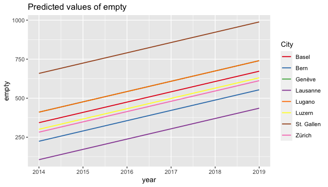
The effect of time on housing is statistically significant for the number of empty housing (positive, with an estimate of 66 additional empty units of housing each year between 2014 and 2019, p<0.001), but not for the number of overcrowded housing units. Housing surface also seems to decrease slightly by 0.054 square meter per person per year during that period, but the effect is not quite statistically significant (p=0.055).
5. Conclusion
At the descriptive stage, one could observe that the overall values for wooded and recreational area per person per city were relatively constant over the four periods. There was however a slight general trend, as that type of area seemed to increase from 1985 to 2009, before the 2018 mean went back to 1997 levels. Was this a consequence of the 2012/2013 votes, as cities became more densely built to spare the countryside? Although a more complex temporal analysis (specifically, a non-linear one) would be required to evaluate further whether the latest measures deviate from a certain trend, our analysis could already highlight certain elements.
The most parsimonious model, and the one holding the most explanatory power, was the one which included time, population, and language as fixed effects, next to Cantons as random effect. Over the first 3 periods, time is statistically significant, suggesting a positive trend in wooded and recreational area per person in Swiss cities between 1985 and 2009. Overall, an increase in population might have a negative effect on the surface of wooded and recreational area per person, although no model returned quite a statistically significant result for that predictor. Further research would here be necessary to examine in greater detail the interaction between the supposed effect of the 2012/2013 votes and population. In terms of housing, the number of empty housing has been statistically significantly rising from 1985 to 2018, perhaps following a longer trend expectation of greater urbanization, something which might also affect building densification in cities. Housing surface also seems to decrease, but a more detailed approach would be needed to determine whether the trend is accelerating post-2013.
In light of the apparent methodological limitations of the present research, we remain prudent and decide not to propose any definitive answer regarding the evolution of the observed aspects of livability in Swiss cities since 2013. Still, further research, both using more advanced statistical tools and integrating other economical and sociological control variables, could very well build upon our initial findings, the latter indicating that Swiss Cantons, no matter their linguistic character, were evolving towards greater wooded and recreational area per capita between 1985 and 2009, that the housing situation in the largest cities testifies to an expectation of continued urbanization over the last 7 years, and that housing surface per person might be shrinking in urban centers.
References:
Land use data: https://www.bfs.admin.ch/bfs/de/home/statistiken/raum-umwelt/bodennutzung-bedeckung.assetdetail.11007207.html
Housing data: https://www.pxweb.bfs.admin.ch/ , under Stadt / Agglomeration.
Lebensqualität in den Städten und Agglomerationen (Agglo 2012). Bundesamt fuer Statistik, 2019.
Heidegger, Martin. “Building Dwelling Thinking,” in: Poetry, Language, Thought, trans. A. Hofstadter, New York: Harper Colophon Books, 1971.
Co-Director
Global Governance Centre
Professor
International Relations and Political Science
President
Global Governance Research Centre Consortium
International institutions and political networks.