Building Our Way Out of the Crisis: Do Building Characteristics Affect a Neighborhood's Median Rents?
Vladimir Borodin - Statistics for International Relations Research II
- Introduction, Research Question & Hypotheses
- Data
- Methodology / Model
- Results
- Robustness: Eliminating Continuous Aggregated Building Variables
- Conclusion
- References:
Introduction, Research Question & Hypotheses
Of all the devastating effects brought about by the global Covid-19 pandemic in 2020, one positive effect that some home buyers might have been excited for was a drop in rental and purchase prices of housing, following the exodus of people out of global cities like New York. Despite a modest dip in prices, rents in New York City are already on the uptick, suggesting that the drop in demand due to more people working remotely in other cities has not put a dent in the overwhelming demand to live in New York. In this blog post, I try to look at one aspect of the question “Why is the rent so high?” I am curious to see if the intrinsic qualities of the buildings in the various neighborhoods of Brooklyn, NY have any effect on the median rents in their area.
This blogpost mainly addresses the claims made by the “Market Urbanism” and “Yes in my Backyard” (YIMBY) movements in the United States, which argue that addressing the supply of housing (that is, building as many houses as possible) is the solution to the affordable housing shortage in the country. They argue that cities in the US have too many regulations, such as height and lot size restrictions, limiting what type of apartment buildings can be built (Lewyn 2018). While deregulation and expansion of the housing supply may sound intuitive, progressives in the “New Urbanism” camp argue that deregulated housing would lead to displacement of poorer people in the process of gentrification (Robinson 2021).
In this blogpost, I seek to investigate the claim that newer, taller buildings can decrease median rents by looking at cross-sectional data of 744 census tracts in Brooklyn, NYC.
Research Question:
“Do the intrinsic characteristics of buildings in a neighborhood affect that neighborhood’s median rents?”
Hypotheses:
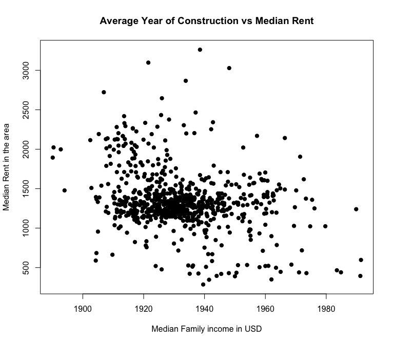
H1: I predict a convex parabolic relationship between the average year that buildings were built in the census tract and the median rent. I assume this will be the case because many home buyers will place a premium on very old buildings, such as those built between 1880-1915 because of the luxurious details and historical value of the homes themselves. I expect the lowest prices to be for apartments in buildings from 1930-1970. After 1990, I expect median rents to increase due to the proliferation of “luxury” apartment buildings.
H2: I predict a positive linear relationship between the average number of floors in a tract and median rents because I suppose taller buildings can charge higher rents for better views.
H3: I predict a positive linear relationship between the number of new residential units (since 1990) constructed in a tract and the median rent in that tract. I believe the new units constructed in these tracts will drive up the median rent, even if those new residences may possibly reduce rents for the city as a whole.
H4: I predict a positive linear relationship between buildings designated as historic and median rents for the same reasons as H1.
H5: I predict a negative linear relationship between median rent and neighborhoods that have at least one public housing building.
Data
I use cross-sectional data for 744 neighborhoods in Brooklyn, NYC in 2016, composed of two datasets. The first is a dataset tracking median rents and population characteristics of census tracts in Brooklyn, compiled by Glen Johnson of the City University of New York School of Public Health. The second is a dataset known as PLUTO, containing the characteristics of 800,000 individual buildings in the city, which I downloaded from the New York City Planning Department’s BYTES of the Big Apple data repository.
Because managing 800,000 observations is extremely difficult, I chose to focus on the borough of Brooklyn. I believe Brooklyn is representative of the rest of the city, and of many North American cities in general, as it is very diverse in building variety and popularity of neighborhoods. Moreover, Brooklyn is at the “front line” of gentrification in the city. For example, the historically Black neighborhood of Bedford-Stuyvesant, made famous by Spike Lee’s “Do the Right Thing” and for its slogan “Bed-Stuy do or die” has had a massive influx of wealthy, mostly-white residents, raising prices in the surrounding area and pricing out its original residents.
In order to put the datasets together, I aggregated all of the buildings into each of Brooklyn’s 744 Federal Information Processing System (FIPS) tracts by either taking the average values or the sums of values of each building in the tract. I then filtered out all non-residential buildings so that the only ones in the data were buildings with at least one residence. I made some of my own variables using Excel pivot tables and IF functions.
One issue I immediately ran into with the data is that it does not differentiate between RENTED and OWNED properties. The variables in this data include ALL residences, and not just rentable apartments. This may explain why rents appear slightly lower than one might expect for Brooklyn, as mortgage payments on properties are not included in the median rents variable.
I thus decided to create my own, separate dataset using the same variables but with single family homes removed. I did this by going back to the original excel file with the 260,000 residential buildings in Brooklyn and removing the 64,000 homes that had only one residential unit per building. This was about the closest approximation of the difference between rented apartments (which have more than one residential unit per building) and single family homes, which typically are not rented, that I could think of. This way, the new dataset I built has exluded many properties that are not on the rental market, and which can skew the results.
All of the variables described below are by FIPS census tract for the year 2016 unless otherwise stated.
Dependent Variable
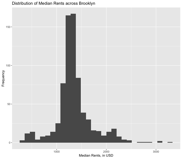
Median Rents: The median rental price for residential units in the FIPS census tract in 2016, as calculated from the 2016 American Community Survey.
##
##  Shapiro-Wilk normality test
##
## data:  sf$mdrent
## W = 0.90085, p-value < 0.00000000000000022
The above histogram shows a relatively normally distribution for the dependent variable, although the Shapiro-Wilkes test rejects the null hypothesis that it is normal. Nevertheless, the law of large numbers allows us to assume that the median rents distribution is approaching normality. Besides, a non-normal dependent variable does not violate the assumptions of a Best, Linear, Unbiased Estimator model for Ordinary Least Squares Regression.
Independent Variables
totpop: The total population in the tract.
popover24: The population over 24 years old.
whitepop: Total non-Hispanic White population.
20-34pop: The population between 20-34 years old.
collegepop: The population with a college degree.
mdfamincome: The median family income, in USD.
avglandvalue: The average assessed land value of the land under the buildings in the tract, in USD. The NYC Department of Finance calculates assessed value by multiplying the building’s estimated full market land value, determined as if vacant and unimproved, by a uniform percentage for the property’s tax class. This and the following variables were aggregated using Excel Pivot tables.
avgfar: The average Floor Area Ratio (FAR) of buildings in the tract. FAR is calculated as the total building floor area divided by the area of the tax lot. Because this is a ratio, it remains the same regardless of which units of measurement are used.
avgyear: The average year of construction for all the residential buildings in the tract. This is transformed to have a mean centered at zero as otherwise it would lead to wildly high intercept estimates.
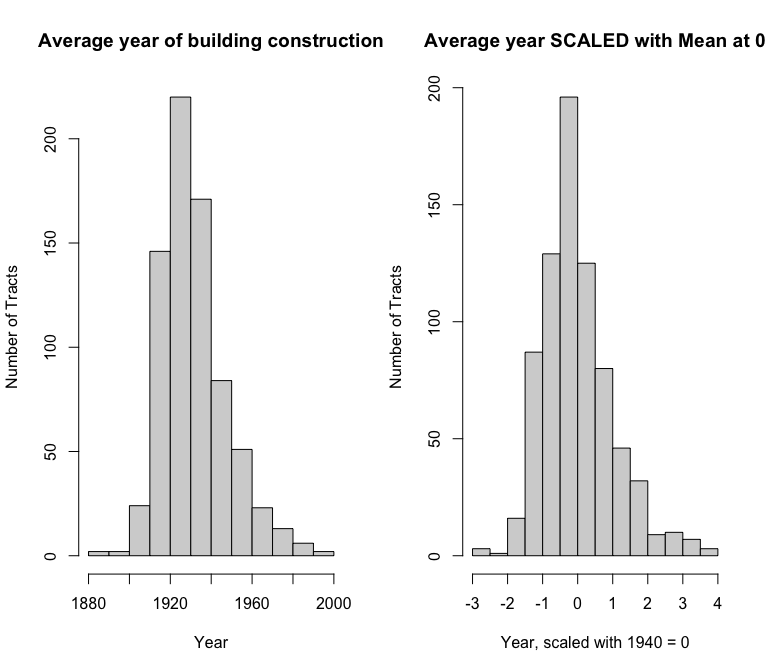
The above side-by-side histograms show the distribution of the average year of construction for buildings in each of the 744 FIPS tracts. On the right, I have scaled the year variable by subtracting from it the mean year, and then dividing by the standard deviation, to center the distribution around 0.
avgarea: The average size of the buildings in a tract, in squared feet. Total area per building is calculated by adding together the usable squared area of each floor in a residential building. I take the average total area per building. Amenities and common spaces are included, but rooftop spaces are not.
avgunitsres: The average number of residential units per building per tract.
totalbldgs: The total number of residential buildings. This is calculated by taking the sum of all buildings in a FIPS area using an Excel Pivot table.
histbldgs: The total number of buildings with a historical designation per tract.
historic: A binary dummy variable coded to be 1 if there are any designated historical buildings in the tract and 0 if there are none.
renovbldgs: The total number of buildings renovated since 1990 per tract.
pbauthbldgs: The total number of buildings designated as belonging to a public authority per tract. This is a proxy variable for affordable housing projects owned by the NYC Housing Authority. I am making this assumption because I cannot think of any other public agency that owns residential buildings in NYC.
pbauth: A binary dummy variable coded to be 1 if there are any residential buildings owned by a public authority in the tract and 0 if there are none.
avgfloors: The average number of floors per building per tract.
newbldgs: The total number of residential buildings built since 1990 per tract.
newresid: The total number of residential units in buildings built since 1990 per tract.
## [1] "<table class=\"Rtable1-zebra\">\n<thead>\n<tr>\n<th class='rowlabel firstrow lastrow'></th>\n<th class='firstrow lastrow'><span class='stratlabel'>Overall<br><span class='stratn'>(N=744)</span></span></th>\n</tr>\n</thead>\n<tbody>\n<tr>\n<td class='rowlabel firstrow'><span class='varlabel'>Total Population</span></td>\n<td class='firstrow'></td>\n</tr>\n<tr>\n<td class='rowlabel'>Mean (SD)</td>\n<td>3490 (1380)</td>\n</tr>\n<tr>\n<td class='rowlabel lastrow'>Median [Min, Max]</td>\n<td class='lastrow'>3330 [432, 8950]</td>\n</tr>\n<tr>\n<td class='rowlabel firstrow'><span class='varlabel'>Population 24+</span></td>\n<td class='firstrow'></td>\n</tr>\n<tr>\n<td class='rowlabel'>Mean (SD)</td>\n<td>2350 (926)</td>\n</tr>\n<tr>\n<td class='rowlabel lastrow'>Median [Min, Max]</td>\n<td class='lastrow'>2260 [256, 5820]</td>\n</tr>\n<tr>\n<td class='rowlabel firstrow'><span class='varlabel'>Non-Hispanic White Population</span></td>\n<td class='firstrow'></td>\n</tr>\n<tr>\n<td class='rowlabel'>Mean (SD)</td>\n<td>1250 (1200)</td>\n</tr>\n<tr>\n<td class='rowlabel lastrow'>Median [Min, Max]</td>\n<td class='lastrow'>1030 [0, 8480]</td>\n</tr>\n<tr>\n<td class='rowlabel firstrow'><span class='varlabel'>Population between age 20-34</span></td>\n<td class='firstrow'></td>\n</tr>\n<tr>\n<td class='rowlabel'>Mean (SD)</td>\n<td>880 (451)</td>\n</tr>\n<tr>\n<td class='rowlabel lastrow'>Median [Min, Max]</td>\n<td class='lastrow'>798 [26.0, 2960]</td>\n</tr>\n<tr>\n<td class='rowlabel firstrow'><span class='varlabel'>People with College Degree</span></td>\n<td class='firstrow'></td>\n</tr>\n<tr>\n<td class='rowlabel'>Mean (SD)</td>\n<td>802 (604)</td>\n</tr>\n<tr>\n<td class='rowlabel lastrow'>Median [Min, Max]</td>\n<td class='lastrow'>628 [49.0, 3670]</td>\n</tr>\n<tr>\n<td class='rowlabel firstrow'><span class='varlabel'>Median Family Income, USD</span></td>\n<td class='firstrow'></td>\n</tr>\n<tr>\n<td class='rowlabel'>Mean (SD)</td>\n<td>67000 (34100)</td>\n</tr>\n<tr>\n<td class='rowlabel lastrow'>Median [Min, Max]</td>\n<td class='lastrow'>59500 [14500, 248000]</td>\n</tr>\n<tr>\n<td class='rowlabel firstrow'><span class='varlabel'>Median Rent, USD</span></td>\n<td class='firstrow'></td>\n</tr>\n<tr>\n<td class='rowlabel'>Mean (SD)</td>\n<td>1350 (375)</td>\n</tr>\n<tr>\n<td class='rowlabel lastrow'>Median [Min, Max]</td>\n<td class='lastrow'>1300 [286, 3260]</td>\n</tr>\n<tr>\n<td class='rowlabel firstrow'><span class='varlabel'>Total Buildings</span></td>\n<td class='firstrow'></td>\n</tr>\n<tr>\n<td class='rowlabel'>Mean (SD)</td>\n<td>298 (153)</td>\n</tr>\n<tr>\n<td class='rowlabel lastrow'>Median [Min, Max]</td>\n<td class='lastrow'>299 [3.00, 1090]</td>\n</tr>\n<tr>\n<td class='rowlabel firstrow'><span class='varlabel'>Residences in New Buildings</span></td>\n<td class='firstrow'></td>\n</tr>\n<tr>\n<td class='rowlabel'>Mean (SD)</td>\n<td>125 (259)</td>\n</tr>\n<tr>\n<td class='rowlabel lastrow'>Median [Min, Max]</td>\n<td class='lastrow'>43.0 [0, 4160]</td>\n</tr>\n<tr>\n<td class='rowlabel firstrow'><span class='varlabel'>New Buildings, since 1990</span></td>\n<td class='firstrow'></td>\n</tr>\n<tr>\n<td class='rowlabel'>Mean (SD)</td>\n<td>17.7 (29.9)</td>\n</tr>\n<tr>\n<td class='rowlabel lastrow'>Median [Min, Max]</td>\n<td class='lastrow'>7.00 [0, 366]</td>\n</tr>\n<tr>\n<td class='rowlabel firstrow'><span class='varlabel'>Units owned by Public Authority</span></td>\n<td class='firstrow'></td>\n</tr>\n<tr>\n<td class='rowlabel'>Mean (SD)</td>\n<td>80.7 (316)</td>\n</tr>\n<tr>\n<td class='rowlabel lastrow'>Median [Min, Max]</td>\n<td class='lastrow'>0 [0, 2880]</td>\n</tr>\n<tr>\n<td class='rowlabel firstrow'><span class='varlabel'>Average Floor Area Ratio (FAR), feet squared</span></td>\n<td class='firstrow'></td>\n</tr>\n<tr>\n<td class='rowlabel'>Mean (SD)</td>\n<td>1.79 (0.854)</td>\n</tr>\n<tr>\n<td class='rowlabel lastrow'>Median [Min, Max]</td>\n<td class='lastrow'>1.68 [0, 10.0]</td>\n</tr>\n<tr>\n<td class='rowlabel firstrow'><span class='varlabel'>Total Historical Buildings</span></td>\n<td class='firstrow'></td>\n</tr>\n<tr>\n<td class='rowlabel'>Mean (SD)</td>\n<td>14.3 (56.0)</td>\n</tr>\n<tr>\n<td class='rowlabel lastrow'>Median [Min, Max]</td>\n<td class='lastrow'>0 [0, 482]</td>\n</tr>\n<tr>\n<td class='rowlabel firstrow'><span class='varlabel'>Buildings Renovated since 1990</span></td>\n<td class='firstrow'></td>\n</tr>\n<tr>\n<td class='rowlabel'>Mean (SD)</td>\n<td>1.81 (2.62)</td>\n</tr>\n<tr>\n<td class='rowlabel lastrow'>Median [Min, Max]</td>\n<td class='lastrow'>1.00 [0, 22.0]</td>\n</tr>\n<tr>\n<td class='rowlabel firstrow'><span class='varlabel'>Average Year of Building Construction</span></td>\n<td class='firstrow'></td>\n</tr>\n<tr>\n<td class='rowlabel'>Mean (SD)</td>\n<td>1930 (15.5)</td>\n</tr>\n<tr>\n<td class='rowlabel lastrow'>Median [Min, Max]</td>\n<td class='lastrow'>1930 [1890, 1990]</td>\n</tr>\n<tr>\n<td class='rowlabel firstrow'><span class='varlabel'>Average Land Value, USD</span></td>\n<td class='firstrow'></td>\n</tr>\n<tr>\n<td class='rowlabel'>Mean (SD)</td>\n<td>130000 (633000)</td>\n</tr>\n<tr>\n<td class='rowlabel lastrow'>Median [Min, Max]</td>\n<td class='lastrow'>18500 [4980, 6690000]</td>\n</tr>\n<tr>\n<td class='rowlabel firstrow'><span class='varlabel'>Average Amount of Residential Units per Building</span></td>\n<td class='firstrow'></td>\n</tr>\n<tr>\n<td class='rowlabel'>Mean (SD)</td>\n<td>29.8 (144)</td>\n</tr>\n<tr>\n<td class='rowlabel lastrow'>Median [Min, Max]</td>\n<td class='lastrow'>4.30 [2.00, 1590]</td>\n</tr>\n<tr>\n<td class='rowlabel firstrow'><span class='varlabel'>Average Floors per Building</span></td>\n<td class='firstrow'></td>\n</tr>\n<tr>\n<td class='rowlabel'>Mean (SD)</td>\n<td>2.97 (2.01)</td>\n</tr>\n<tr>\n<td class='rowlabel lastrow'>Median [Min, Max]</td>\n<td class='lastrow'>2.53 [1.16, 24.0]</td>\n</tr>\n<tr>\n<td class='rowlabel firstrow'><span class='varlabel'>avgyearscaled</span></td>\n<td class='firstrow'></td>\n</tr>\n<tr>\n<td class='rowlabel'>Mean (SD)</td>\n<td>0.00000000000000213 (1.00)</td>\n</tr>\n<tr>\n<td class='rowlabel lastrow'>Median [Min, Max]</td>\n<td class='lastrow'>-0.123 [-2.70, 3.83]</td>\n</tr>\n<tr>\n<td class='rowlabel firstrow'><span class='varlabel'>avgyearsq</span></td>\n<td class='firstrow'></td>\n</tr>\n<tr>\n<td class='rowlabel'>Mean (SD)</td>\n<td>0.999 (1.69)</td>\n</tr>\n<tr>\n<td class='rowlabel lastrow'>Median [Min, Max]</td>\n<td class='lastrow'>0.358 [0.000000953, 14.7]</td>\n</tr>\n<tr>\n<td class='rowlabel firstrow'><span class='varlabel'>historic</span></td>\n<td class='firstrow'></td>\n</tr>\n<tr>\n<td class='rowlabel'>Mean (SD)</td>\n<td>0.109 (0.312)</td>\n</tr>\n<tr>\n<td class='rowlabel lastrow'>Median [Min, Max]</td>\n<td class='lastrow'>0 [0, 1.00]</td>\n</tr>\n<tr>\n<td class='rowlabel firstrow'><span class='varlabel'>pbauth</span></td>\n<td class='firstrow'></td>\n</tr>\n<tr>\n<td class='rowlabel'>Mean (SD)</td>\n<td>0.130 (0.337)</td>\n</tr>\n<tr>\n<td class='rowlabel lastrow'>Median [Min, Max]</td>\n<td class='lastrow'>0 [0, 1.00]</td>\n</tr>\n</tbody>\n</table>\n"

## [1] 0
Comments
The data I’m working with is impressive because it contains no missing values, attesting to the good record keeping of the NYC Department of City Planning. Moreover, as one can see in the table above, the total population of each FIPS tract does not vary too much, meaning we are comparing like with like.
Unfortunately, the plots below do not bode well for investigation:
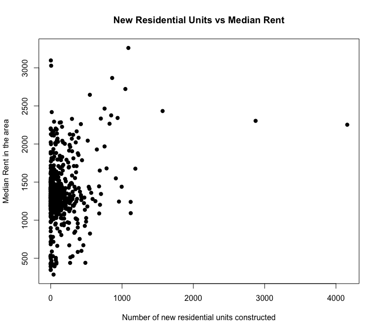
One of the key variables of interest, new residential units constructed per tract, is clustered around 0, creating a distribution that does not appear to have much effect on median rents.
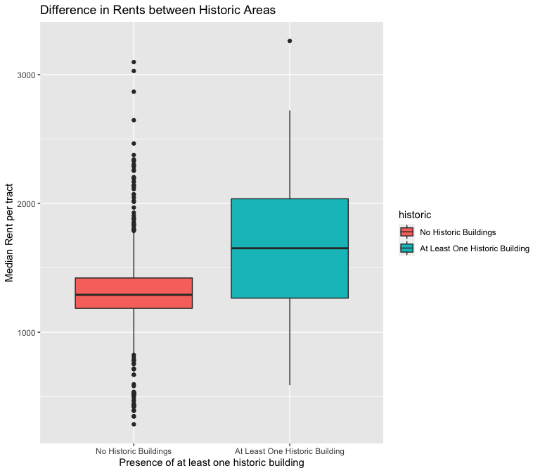
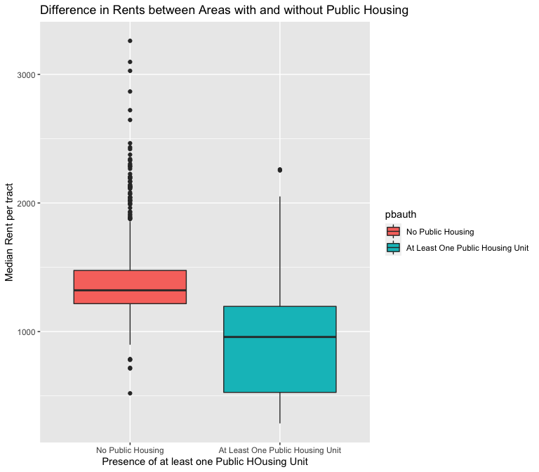
The above box plots look more promising, as they suggest that FIPS tracts with at least one historic building have higher rents and tracts with at least one unit of public housing have lower rents.
Relationships in the Data
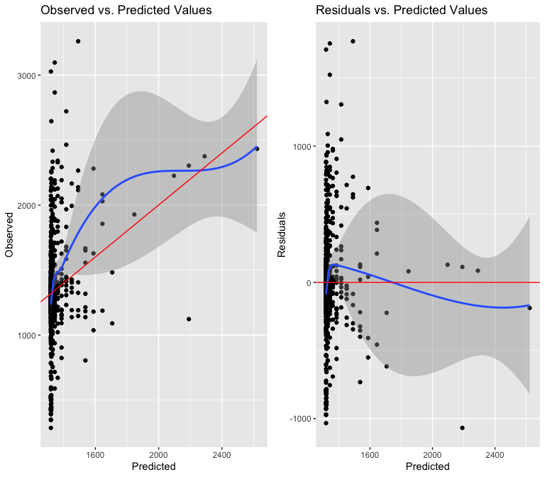
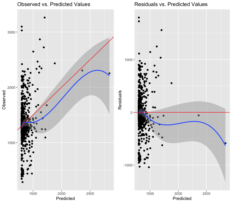
Because I want to use an ordinary least squares model, I need to make sure that it is adherent to the Gauss Markov assumptions. The first requirement is that my model is linear in its parameters. That means I first want to test the linearity of the relationship between median rents and my first variable of interest: year of construction.
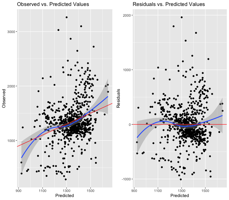
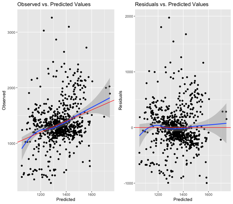
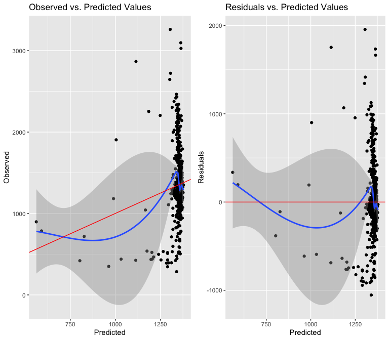
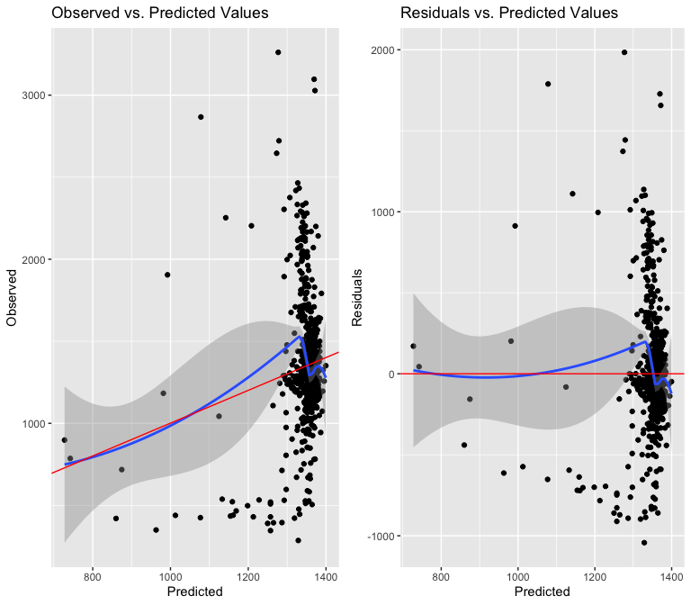
Above, I noticed that the year term had a bow shape at the beginning and end of the distribution of observed and residual values vs the predicted values. I thought that squaring the term might make the relationship more linear, because my hypothesis was that the relationship between year and median rent would be parabolic. The second two graphs disprove my theory, because the bow shape gets even worse with a squared term. I believe this variable is still worth testing however, and it appears it is more linear than I supposed.
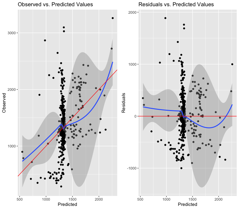
The next variable I will test is the average amount of floors in an
area:
I try to correct for the bow shape by using a squared term, but I see that the relationship is not in any way close to linear, especially because the values cluster so much at the end of the x axis. I will try to use an interaction term, though I am skeptical this will amount to anything, since an interaction term cannot fix the underlying non-linearity.
As I expected, including a term for the interaction between tracts with at least one historically designated building and the average amount of floors does not address the issue of non-linearity. Moreover, if I look at the residuals vs predicted values plot, I see two funnel shapes in the distribution, which suggests heteroskedasticity.
The Breusch-Pagan Test confirms this:
##
##  studentized Breusch-Pagan test
##
## data:  histfloors
## BP = 58.672, df = 3, p-value = 0.00000000000113
The extremely small p-value of the Breusch Pagan test leads me to reject the null hypothesis of homoskedasticity. I believe there is no transformation that I could do to make this relationship linear, so I will not include this variable in the final model. This is unfortunate because I thought an interaction term would be very useful to predicting rents.
Unfortunately, the linearity and heteroskedasticity problems are the
same for the amount of newly renovated buildings in a tract:
As well as the amount of new residential units built in a tract:
##
##  studentized Breusch-Pagan test
##
## data:  resid1
## BP = 18.848, df = 1, p-value = 0.00001415
Both the renovated buildings and new residential units variables are too non-linear and heteroskedastic to justify using in a predictive model. I suspect this is because of the overwhelming number of observations that have 0 renovations or new buildings constructed, skewing the distribution towards 0.
Omitted Variable Bias
The distinct clustering pattern on each of the variables tested so far hints at a possible omitted variable, justifying a Ramsey RESET test to check for endogeneity concerns:
##
##  RESET test
##
## data:  resid1
## RESET = 3.8392, df1 = 2, df2 = 740, p-value = 0.02194

##
##  RESET test
##
## data:  histfloors
## RESET = 0.68386, df1 = 2, df2 = 738, p-value = 0.505
The first test allows us to reject the null hypothesis that a model with additional polynomial terms is equally well-specified as the model with just new residential units as a predictor. This means the explanatory power of new residential unit construction would increase if some omitted variable were added to it, giving me further proof that I should not include either of these variables in the final model.
Methodology / Model
I propose to use a Ordinary Least Squares model to estimate the effects of building characteristics on median rents. Because I have already ruled out a few variables as violating fundamental assumptions of OLS, I will start with a very parsimonious model using the scaled construction year, the presence of historical buildings and the presence of public authority buildings as the explanatory variables.
Model 1
| Median Rent, USD | |||||
|---|---|---|---|---|---|
| Predictors | Estimates | std. Error | CI | Statistic | p |
| (Intercept) | 1499.29 | 37.93 | 1424.83 – 1573.76 | 39.53 | <0.001 |
| avgyearscaled | -54.80 | 13.67 | -81.64 – -27.96 | -4.01 | <0.001 |
| pbauth: At Least One Public Housing Unit | -388.24 | 46.06 | -478.67 – -297.81 | -8.43 | <0.001 |
| historic: At Least One Historic Building | 277.33 | 57.88 | 163.70 – 390.97 | 4.79 | <0.001 |
| Total Population | -0.04 | 0.01 | -0.06 – -0.02 | -3.85 | <0.001 |
| Observations | 744 | ||||
| R2 / R2 adjusted | 0.279 / 0.275 | ||||
We see that, with robust standard errors, the coefficients of each of the variables are significant at the .01 level. I will interpret substantively the model I choose in the following section.
Model 1: Checking for Normality, Heteroskedasticity, Multicollinearity
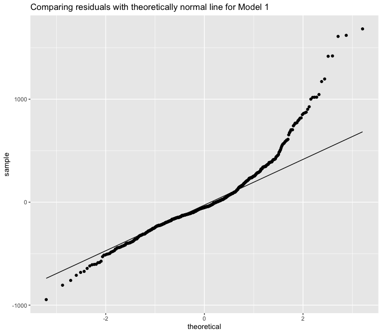
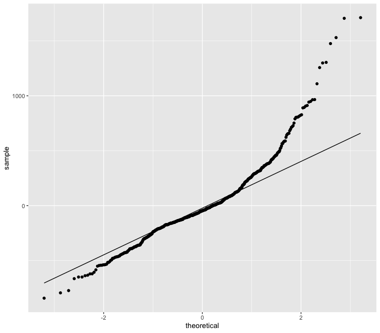
Looking at the Q-Q plot above, I can conclude that this model exhibits kurtosis, since its residuals deviate from a 45 degree “normal” line at both ends of the distribution. This suggests that the model is non-normal in its errors.
## -----------------------------------------------
##        Test             Statistic       pvalue
## -----------------------------------------------
## Shapiro-Wilk               0.91          0.0000
## Kolmogorov-Smirnov        0.1142         0.0000
## Cramer-von Mises         68.4862         0.0000
## Anderson-Darling         16.2416         0.0000
## -----------------------------------------------
The above normality tests confirm my suspicion that this model is non-normal, as all of them are extremely significant. A non-normal model means I cannot make any inferences by performing statistical hypothesis tests.
## Warning: `arrange_()` was deprecated in dplyr 0.7.0.
## Please use `arrange()` instead.
## See vignette('programming') for more help
##
##  studentized Breusch-Pagan test
##
## data:  lm1
## BP = 37.746, df = 4, p-value = 0.0000001264
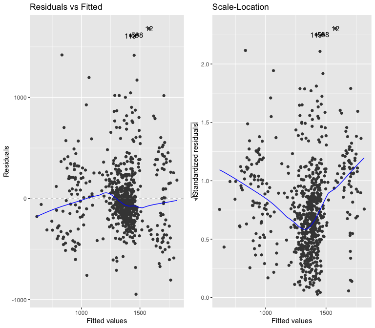
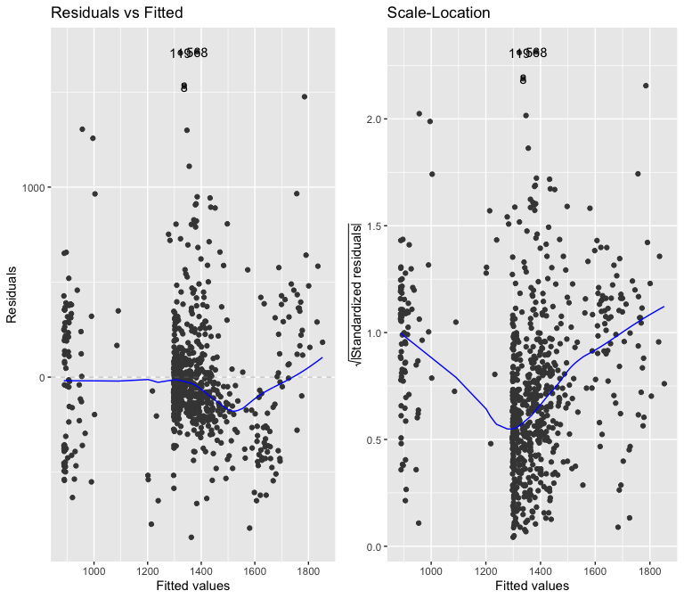
According to the Breusch-Pagan test above, the model is heteroskedastic, which I can confirm by looking at the residuals vs fitted values graph. I will use robust standard errors to try to combat the heteroskedasticity. In my opinion, I the variance in residuals that I observe does not warrant such a low p-value on the Breusch-Pagan test.
##                   [,1]
## avgyearscaled 1.207507
## pbauth        1.093791
## historic      1.175750
## totpop        1.064808
A quick glance above at the Variance Inflation Factor coefficients for each of the explanatory variables tells us there is no multicollinearity in the model, as typically only coefficients with values larger than 4 are cause for worry.
Model 2
I will try taking the log of the response variable to combat the heteroskedasticity problems of model 1.
| Median Rent, USD | |||||
|---|---|---|---|---|---|
| Predictors | Estimates | std. Error | CI | Statistic | p |
| (Intercept) | 7.30 | 0.03 | 7.24 – 7.35 | 260.60 | <0.001 |
| avgyearscaled | -0.06 | 0.01 | -0.08 – -0.03 | -4.95 | <0.001 |
| pbauth: At Least One Public Housing Unit | -0.43 | 0.05 | -0.52 – -0.33 | -8.87 | <0.001 |
| historic: At Least One Historic Building | 0.15 | 0.04 | 0.08 – 0.22 | 4.11 | <0.001 |
| Total Population | -0.00 | 0.00 | -0.00 – -0.00 | -3.50 | <0.001 |
| Observations | 744 | ||||
| R2 / R2 adjusted | 0.369 / 0.366 | ||||
The coefficients in this model are still all significant at the .01 level, but now their magnitudes have changed because of the logged response variable. I will interpret substantively the model I choose in the following section.
Model 2: Checking for Normality, Heteroskedasticity, Multicollinearity
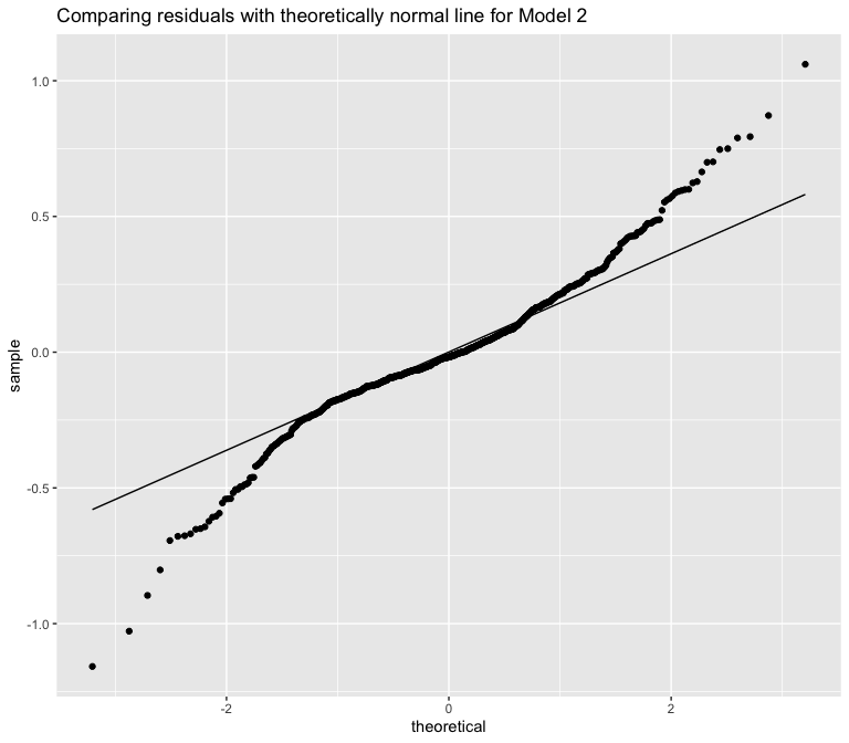
Model 2’s skewness is slightly less than model 1’s, although the kurtosis is still clearly visible.
## -----------------------------------------------
##        Test             Statistic       pvalue
## -----------------------------------------------
## Shapiro-Wilk               0.91          0.0000
## Kolmogorov-Smirnov        0.1142         0.0000
## Cramer-von Mises         68.4862         0.0000
## Anderson-Darling         16.2416         0.0000
## -----------------------------------------------
Even with a logged response variable, all 4 of the above tests show that the model is non-normal.
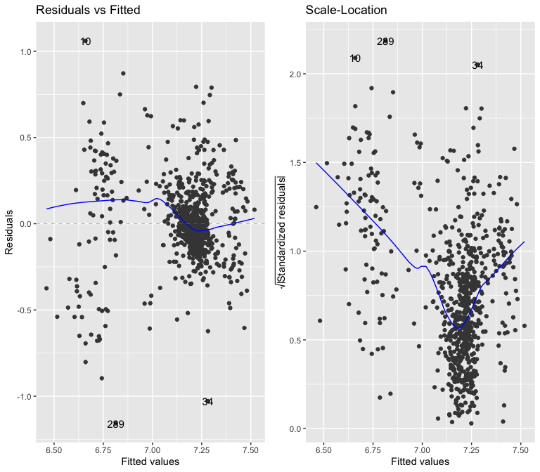
##
##  studentized Breusch-Pagan test
##
## data:  lm2
## BP = 160.96, df = 4, p-value < 0.00000000000000022
The above Breusch-Pagan test is even more conclusively showing that the model is heteroskedastic. I can clearly see that the logging median rents has done nothing to resolve the heteroscedasticity issue.
##                   [,1]
## avgyearscaled 1.207507
## pbauth        1.093791
## historic      1.175750
## totpop        1.064808
At least this model is not collinear.
Model 3
I propose predicting median rents the average year of construction in the tract as an explanatory variable and with median family income as a control. Considering the two last models failed multiple assumptions, I’m hoping this one with only two variables would work.
| Median Rent, USD | |||||
|---|---|---|---|---|---|
| Predictors | Estimates | std. Error | CI | Statistic | p |
| (Intercept) | 855.45 | 25.19 | 805.99 – 904.90 | 33.96 | <0.001 |
| avgyearscaled | -52.64 | 11.10 | -74.43 – -30.84 | -4.74 | <0.001 |
| Median Family Income, USD | 0.01 | 0.00 | 0.01 – 0.01 | 18.81 | <0.001 |
| Observations | 744 | ||||
| R2 / R2 adjusted | 0.509 / 0.507 | ||||
The coefficients of both variables and the intercept are statistically significant at the .01 level.
Model 3: Checking for Normality, Heteroskedasticity, Multicollinearity
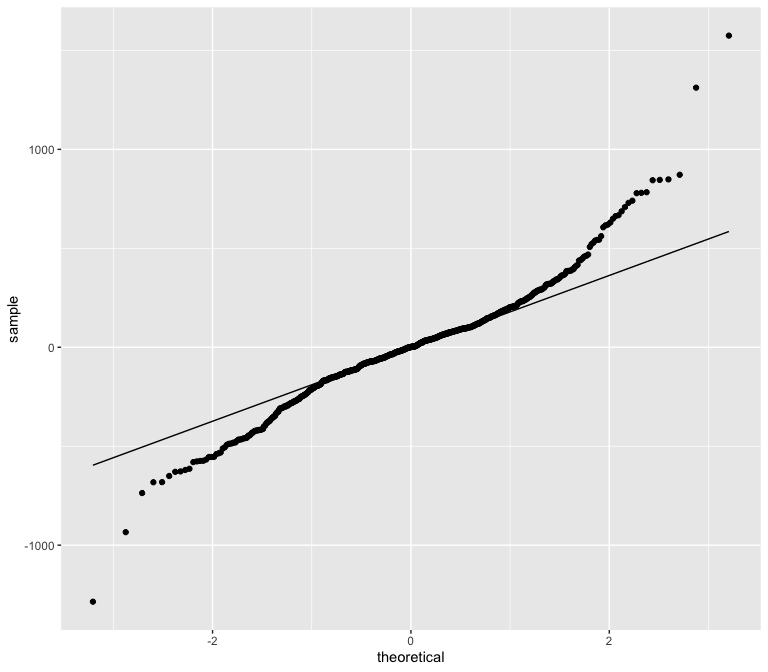
I still see some kurtosis based on the skew at both ends of the Q-Q plot.
## -----------------------------------------------
##        Test             Statistic       pvalue
## -----------------------------------------------
## Shapiro-Wilk               0.91          0.0000
## Kolmogorov-Smirnov        0.1142         0.0000
## Cramer-von Mises         68.4862         0.0000
## Anderson-Darling         16.2416         0.0000
## -----------------------------------------------
I believe there is nothing I can do about the non-normality of the models. It appears that building characteristics aggregated by area will always lead to skewed relationships with median rent.
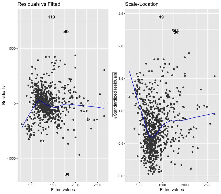
##
##  studentized Breusch-Pagan test
##
## data:  lm3
## BP = 22.882, df = 2, p-value = 0.00001075
Even with only two variables, the model is heteroskedastic.
Model Selection
Although all three of the models have failed fundamental assumptions of linearity, normality, and heteroskedasticity, I believe I should still choose one to interpret by looking for the model with the lowest AIC score and relatively good r squared.
| Median Rent, USD | Median Rent, USD | Median Rent, USD | ||||||||||
|---|---|---|---|---|---|---|---|---|---|---|---|---|
| Predictors | Estimates | std. Error | CI | p | Estimates | std. Error | CI | p | Estimates | std. Error | CI | p |
| (Intercept) | 1499.29 | 37.93 | 1424.83 – 1573.76 | <0.001 | 7.30 | 0.03 | 7.24 – 7.35 | <0.001 | 855.45 | 25.19 | 805.99 – 904.90 | <0.001 |
| avgyearscaled | -54.80 | 13.67 | -81.64 – -27.96 | <0.001 | -0.06 | 0.01 | -0.08 – -0.03 | <0.001 | -52.64 | 11.10 | -74.43 – -30.84 | <0.001 |
| pbauth: At Least One Public Housing Unit | -388.24 | 46.06 | -478.67 – -297.81 | <0.001 | -0.43 | 0.05 | -0.52 – -0.33 | <0.001 | ||||
| historic: At Least One Historic Building | 277.33 | 57.88 | 163.70 – 390.97 | <0.001 | 0.15 | 0.04 | 0.08 – 0.22 | <0.001 | ||||
| Total Population | -0.04 | 0.01 | -0.06 – -0.02 | <0.001 | -0.00 | 0.00 | -0.00 – -0.00 | <0.001 | ||||
| Median Family Income, USD | 0.01 | 0.00 | 0.01 – 0.01 | <0.001 | ||||||||
| Observations | 744 | 744 | 744 | |||||||||
| R2 / R2 adjusted | 0.279 / 0.275 | 0.369 / 0.366 | 0.509 / 0.507 | |||||||||
| AIC | 10698.693 | 23.365 | 10409.379 | |||||||||
Based on the above comparison, I should conclude that model 2 is superior, with its wildly low AIC of 23.365 compared to AICs of over 10,000 for models 1 and 3. I am extremely suspicious of such a low score, as well as of its very reasonable .366 adjusted r squared. I believe the logged response variable may been a type of overspecification which generated such a good result. Despite these suspicions, I will interpret model 2.
The final model equation is thus: log(medianren**t) = α + β1avgyear.scale**d + β2pbaut**h + β3histori**c + β4totpo**p + ϵ
Results
| Median Rent, USD | ||||
|---|---|---|---|---|
| Predictors | Estimates | std. Error | CI | p |
| (Intercept) | 7.30 | 0.03 | 7.24 – 7.35 | <0.001 |
| avgyearscaled | -0.06 | 0.01 | -0.08 – -0.03 | <0.001 |
| pbauth: At Least One Public Housing Unit | -0.43 | 0.05 | -0.52 – -0.33 | <0.001 |
| historic: At Least One Historic Building | 0.15 | 0.04 | 0.08 – 0.22 | <0.001 |
| Total Population | -0.00 | 0.00 | -0.00 – -0.00 | <0.001 |
| Observations | 744 | |||
| R2 / R2 adjusted | 0.369 / 0.366 | |||
| AIC | 23.365 | |||
Unfortunately, this model violates some of the Gauss Markov assumptions for OLS, namely in regards to linearity of parameters, exogeneity and heteroskedasticity. Consequently, the OLS estimators are not BLUE. The variance of the beta coefficients is also biased, meaning I would not be able to conduct any hypothesis testing because the t and F statistics I use are incorrect.
Nevertheless, the OLS estimators are at least consistent and unbiased. Thus, if we wanted to interpret the coefficients on the table above, the effects of the explanatory variables would be the following.
The above table shows us that for every increase in the average year of buildings constructed in the FIPS tract, the median rent will decrease by 100 * .06 = 6%.
Median rents in tracts with at least one unit of public housing should be 43% lower than in tracts without any public housing.
Tracts with at least one historically designated residential structure should have 15% higher rents than tracts without one.
The coefficient on total population is zero, therefore it is not practically significant as an explanatory variable for median rents.
Robustness: Eliminating Continuous Aggregated Building Variables
As a last resort, I ran a model with only the binary variables of historic and public housing units as well as the total non-hispanic white population. This model did not include any continuous variables from the aggregated building data, so I suspected it could lead to better results.
| Median Rent, USD | |||||
|---|---|---|---|---|---|
| Predictors | Estimates | std. Error | CI | Statistic | p |
| (Intercept) | 1296.97 | 16.92 | 1263.75 – 1330.20 | 76.64 | <0.001 |
| historic: At Least One Historic Building | 296.17 | 50.05 | 197.92 – 394.42 | 5.92 | <0.001 |
| pbauth: At Least One Public Housing Unit | -409.65 | 46.90 | -501.71 – -317.58 | -8.74 | <0.001 |
| Non-Hispanic White Population | 0.06 | 0.01 | 0.03 – 0.08 | 5.03 | <0.001 |
| Observations | 744 | ||||
| R2 / R2 adjusted | 0.275 / 0.272 | ||||
Once again, the coefficients of every variable are significant at the .01 level. I am unsure if this is a result of a mispecified model, or if all the explanatory variables are indeed very signifcant.
Luckily, it appears that the residual vs predicted value distribution only exhibits skewness at the top and not at the bottom of the distribution. This suggests the residuals are close to normally distributed.
## -----------------------------------------------
##        Test             Statistic       pvalue
## -----------------------------------------------
## Shapiro-Wilk              0.914          0.0000
## Kolmogorov-Smirnov        0.1126         0.0000
## Cramer-von Mises          67.198         0.0000
## Anderson-Darling         15.0304         0.0000
## -----------------------------------------------
I am surprised that all 4 of the tests once again assert non-normality. Perhaps my dependent variable is flawed in some way, though I argued earlier that there are enough observations in the data that it should approximate a normal distribution.
##
##  studentized Breusch-Pagan test
##
## data:  lm4
## BP = 30.108, df = 3, p-value = 0.00000131
The model is heteroskedastic, just like the others. I feel like I am out of options for trying different variables or transformations.
Conclusion
Clearly, something was wrong with the underlying data.
Perhaps the issue was in aggregating average values of building characteristics per tract instead of comparing individual buildings. I wanted to see the effects of building characteristics on their neighborhood, and not just on the apartments inside the building being examined. This post was an attempt to see whether constructing tall, new buildings would affect the rents of the surrounding area, and unfortunately the variables I used violated too many of the Gauss Markov assumptions to continue with them. I also tried to keep my models simple without loading them with too many variables to avoid overfitting, yet even then, taking the log of the dependent variable created what I would call a very overfitted model.
Some possible problem sources are:
Omitted Variable Bias: Since heteroskedasticity was rampant in all of my models, I suspect there must be an omitted variable defining the pattern of said distributions. I could not think of instrumental variables because of how neighborhood dynamics usually compound off of each other. More popular neighborhoods will have more construction and probably higher rents; I do not know of a variable that fluctuates with one but not the other, except for policy-level variables which I already had in my model (Historic designation and public housing).
Too many “0” observations: For variables such as historical designated houses or public authority-owned houses, most FIPS tracts had 0 such designations. I believe a Poisson Distribution is the best way to analyze the differences between observations with 0 variables and a small few with large values.
I chose the improper dependent variable to study: I am unsure why this would be the case, since it did not exhibit any strange properties.
Missing Control Variable: Obviously, one of the most important determinants of rent prices in cities is the proximity of an apartment to the city center. My data did not include a variable like this. I could personally have looked at a map and made a judgement on how close each of the 744 tracts are to the city center, but that would have take to long and I doubt it would have fixed the overfitting / heteroskedasticity problems.
This blogpost did not succeed in making any contribution to the YIMBY vs NIMBY debate. However, I still believe the relationship between building characteristics and prices (whether it be rent, or property values) is a promising avenue of further research. Future projects could include looking at how median rents change over time in areas where more new buildings are constructed, compared to areas that do not have much construction. Unfortunately, I did not have access to panel data to test such a claim, but maybe it is possible to find such data sources in the future.
References:
Glaeser, Edward. (2010). Preservation Follies: Excessive landmarking threatens to make Manhattan a refuge for the rich. City Journal Magazine.
Hackworth, J. (2002). Postrecession Gentrification in New York City. Urban Affairs Review, 37(6), 815–843.
Johnson, Glen. (2020) “Data_NYC_Gentrification_2000_16.tab”. Gentrification Index Data for NYC. Harvard Dataverse, V1.
Lewyn, Michael. (2018). The Rise of Market Urbanism. Probate & Property. 32(4)
Newman, K., & Wyly, E. K. (2006). The Right to Stay Put, Revisited: Gentrification and Resistance to Displacement in New York City. Urban Studies, 43(1), 23–57.
NYC Department of City Planning. (2021). PLUTO Data Dictionary. BYTES of the Big Apple.
Robinson, Nathan. (2021). The Only Thing Worse than a NIMBY is a YIMBY. Current Affairs.
Co-Director
Global Governance Centre
Professor
International Relations and Political Science
President
Global Governance Research Centre Consortium
International institutions and political networks.