Agnese Zucca
- 1. Electoral Discrimination in Switzerland
- 1.1 Introduction and Research Question
- 1.2 Hypothese
- 2. Data and Measurement
- 2.1 Study Setting, Data Source and Characteristics
- 2.2 Data, Coding, and Measurement
- 3. Methods
- 4. Results
- 4.1 Overview
- 4.2 Model Selection
- 4.3 Diagnostics
- 4.4 Results
- 5. Conclusion
- References:
1. Electoral Discrimination in Switzerland
1.1 Introduction and Research Question
Switzerland has one of the highest shares of foreign-born population in Europe (Nguyen 2016). In 2018, the number of foreign-born represented 29.65% of the population (OFS 2019a) and 37.5% of the Swiss population aged 15 or above had an immigration background. Of these, 13.6% held a Swiss passport (OFS 2019b). Yet, in recent years Switzerland has also been on the spotlight for the anti-immigration attitudes of its citizens expressed via popular initiatives aimed at imposing restrictions in the immigration domain. This apparent tension raises the question of whether the diversity of the Swiss population is mirrored in its political institutions.
The underrepresentation of immigrant minorities in parliaments is a common characteristic of many European states although it is precisely in democratic countries that institutions should be representative of their populations. Regardless of its causes, underrepresentation may thus be seen as entailing a democratic deficit (Bloemraad and Schönwälder 2013).
In Switzerland, this question has been studied from the discriminatory voting behavior standpoint by Portmann and Stojanović (2019), who found that immigrant-origin candidates received significantly more negative preference votes than their Swiss counterparts in Zurich local elections. This study will assess whether these findings can be extended to the federal level by answering the following research question:
RQ: To what extent does the origin of a candidate influences its chances of success in Swiss parliamentary elections?
1.2 Hypotheses
Voters inferences about the ethnic origins of a candidate have been found to be used as heuristic tools during elections (McDermott 1999). Yet, the specific mechanism explaining how the origin of a candidate influences voters’ evaluations are multiple: voters may simply hold negative attitudes towards immigrants, they could use ethnicity to infer the ideological leaning of a candidate (Street 2014), or they could make evaluations based on the perceived capacity of such candidates to conform to Swiss political culture. The use of a statistical method does not allow to directly test any of such mechanisms. However, the following hypothesis can be formulated:
H1a: Having an immigration background negatively influences the chances of election of a candidate.
2 Data and Measurement
2.1 Study Setting, Data Source and Characteristics
Cross-sectional data on the 2019 federal elections of the National Council (NC) are employed to test the hypothesis. The NC is the lower chamber of the Swiss parliament, it has 200 seats allocated proportionally to the population of Cantons, which serve as electoral districts. The NC is elected with an open-PR system (except in the six cantons that only have one seat, who elect their representatives through a majoritarian system). The main source of data employed for the analysis is an official dataset compiled by the Federal Statistical Office (Opendata.swiss 2019) that includes several personal information on candidates. The final dataset includes information on 4,664 candidates, who represent the unit of analysis (four observations in the original dataset have been deleted because they were aggregates not corresponding to a specific candidate).
library(utils)
elections<- read.csv2("/Users/Juliette/Dropbox/Stats II/Assignments (1)/Final project/Agnese Cecilia Maria Zucca_114354_assignsubmission_file_/CN2019.csv", header=TRUE, dec=".")
2.2 Data, Coding, and Measurement
Response Variable and Main Independent Variables
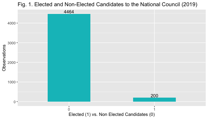
The dependent variable electoral success is a categorical bianry variable where 0 indicates non-election and 1 election. The barplot in Fig. 1 displays its distrubution.
library(ggplot2)
library(scales)

ggplot (data=elections, aes(x = factor(elected))) + geom_bar(position="dodge",  fill="#00BFC4", width=0.5) + xlab("Elected (1) vs. Non Elected Candidates (0)") +
    ylab("Observations") + ggtitle("Fig. 1. Elected and Non-Elected Candidates to the National Council (2019)") + geom_text(stat = 'count', aes(label = stat(count), vjust = -0.2))
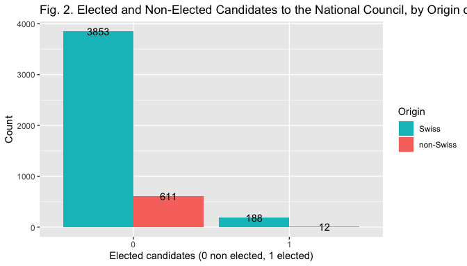
The measure the main independent variable origin of the candidate the origin of family names of candidates is considered. The use of names to determine candidates’ origin has been employed in similar studies and the rationale behind it is that names provide voters with an information cue regarding the origin of the candidate, and may thus be used as a heuristic tool when casting votes (Portmann and Stojanović 2019; Thrasher et al. 2015). First, each of the 4,664 names has been coded according to which it was Swiss or not. Following Portmann and Stojanović (2019) all family names appearing in the Register of Swiss Family Names (RSS 2020) as bore by someone with Swiss citizenship before 1940 have been coded as Swiss (see Portmann and Stojanovicc2ć for a discussion of the cut-off). All the other names have been coded as “non-Swiss”. This results in a categorical binary measure (0 = Swiss name, 1 = non-Swiss name). As highlighted by Stojanović and Portmann (2019), this coding procedure is not necessarily precise, as Swiss candidates that through marriage acquire a foreign family name or foreign ones that acquire Swiss names would be misclassified. However, the misscategorization is less worrisome if one considers that voters infer the origin from names and use them as heuristic tools.
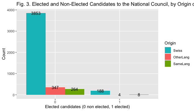
To conduct robustness checks comparable to the ones of Stojanović and Portmann (2019) their approach has been further followed to create two additional measures of name origin. The country or region of non-Swiss names has been coded using the database “forebears.io” (as well as background information available on the internet and first names when in doubt). For the first additional measure, names have been classified as either Swiss, Non-Swiss but linguistically proximate to Switzerland (i.e. IT, FR, D and AT) or Non-Swiss but linguistically distant (i.e. all the rest). The measure was chosen by the authors to account for the potential inability to discriminate between Swiss and other linguistically proximate names. Further, voters may also consider that coming from a neighbouring country and speaking the same language facilitates integration, and thus consider these candidates better equipped than other foreigners to serve as MPs. For the second, names have been classified as Swiss, Western (i.e. Western, Southern and Northern Europeans and Anglo-Saxon names) or Non-Western (i.e. Eastern European, Western Balkans, Turkish, Asian, African and Latin American names). This distinction has been included considering that the strenght of immigration prejudices may vary: western individuals may be perceived more similar to Swiss ones, and thus be suject to less prejudice than non-Western ones. Both variables are categorical and take three values (0 if Swiss, 1 if linguistically proximate/Western, 2 if linguistically distant/non-Western).
The bar plot in Fig. 2, 3 and 4 help visualize the relationship between the election outcome and the different measures of the indipendent variables.
library(ggplot2)
library(scales)

ggplot (data=elections, mapping = aes(x = factor(elected), fill = factor(nameorigin)))+ geom_bar(position='dodge') + xlab("Elected candidates (0 non elected, 1 elected)") +
    ylab("Count") + ggtitle("Fig. 2. Elected and Non-Elected Candidates to the National Council, by Origin of Family Name (2019)") + labs (fill="Origin") + geom_text(stat = 'count', aes(label = stat(count)), position=position_dodge(width = 0.9)) + scale_fill_manual(values=c("#00BFC4", "#F8766D"), labels=c("Swiss", "non-Swiss"))
elections$nameoriginl <- relevel(elections$nameoriginl, ref = "Swiss")
elections$nameoriginw <- relevel(elections$nameoriginw, ref = "Swiss")

ggplot (data=elections, mapping = aes(x = factor(elected), fill = factor(nameoriginl))) + geom_bar(position="dodge") + xlab("Elected candidates (0 non elected, 1 elected)") + ylab("Count") + ggtitle("Fig. 3. Elected and Non-Elected Candidates to the National Council, by Origin of Family Name") + labs (fill="Origin") + geom_text(stat = 'count',  aes(label = stat(count)), position=position_dodge(width = 0.9)) + scale_fill_manual(values=c("#00BFC4", "#F8766D", "#7CAE00"))
ggplot (data=elections, mapping = aes(x = factor(elected), fill = factor(nameoriginw)))+ geom_bar(position="dodge") + xlab("Elected candidates (0 non elected, 1 elected)") +
    ylab("Count") + ggtitle("Fig. 4. Elected and Non-Elected Candidates to the National Council, by Origin of Family Name (2019)") + labs (fill="Origin") + geom_text(stat = 'count', aes(label = stat(count)), position=position_dodge(width = 0.9)) + scale_fill_manual(values=c("#00BFC4", "#F8766D", "#7CAE00"))

Other candidates’ individual characteristics that may have an effect on the personal election outcome are included as controls.
Gender is a categorical binary variable (1 if woman, 0 if men). It is included because it is one of the information voters can easily infer from the ballot by looking at names, and may thus use it as a heuristic tool (McDermott 1998, Stojanovic and Portmann 2019).
library(stats)
elections$gender <- relevel(elections$gender, ref="M")
Age Category is a categorical variable with three levels (18-35; 36-60; 61+). It has been created by substracting the year of birth from 2019 at the stage of data coding and subsequently the continuous variable has been binned into the three categories with R. Age is included because it is one of the few information voters possess about the candidate and may thus be used as a cue (Lutz 2010). In addition, older candidates may be favoured over younger ones because they may signal experience and competence.
library(base)
agecat<- cut(elections$age, breaks=c(17, 35, 60, Inf), labels=c("18-35", "36-60", "61+"))
Incumbency Status is a categorical binary variable created by attributing value 1 to incumbents and 0 to the others. Being an incumbent should exert a positive effect on the elction outcome as incumbents are more known to the public and more likely to invest in their campaign (Lutz 2010).
Ballot Position is a numerical variable indicating the position of a candidate name on the ballot (1 = top of the list). Ballot position is included as control as it is deemed to influence election outcomes through name-order effects that provide an advantage to top positions (Lutz 2010; Thrasher 2015). The coefficient is expected to be negative as higher numbers indicate a lower position on the ballot.
Pre Cumulation is a categorical binary variable created by attributing 1 to all individuals holding two list positions and 0 to others. In Switzerland candidates can be listed two times on the same ballot and could hence double their votes. As such, it should exert a positive effect on election outcomes (Lutz 2010).
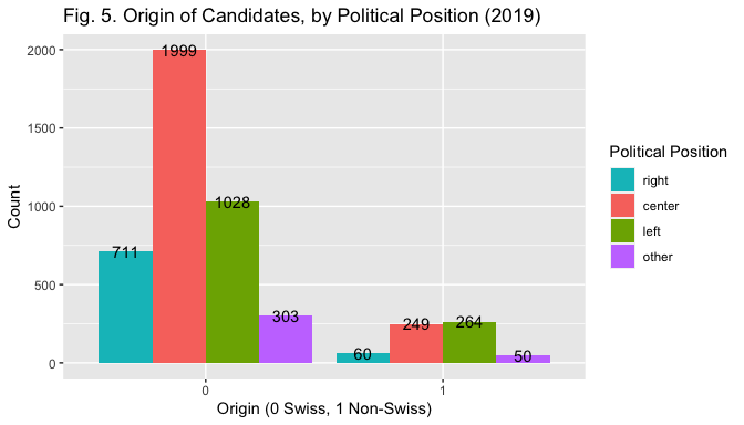
Political Position - Left is a categorical binary variable created by merging the categories center, right and other (= 0) and opposing them to left (=1) (candidates were first coded according to their left, center and right position plus, the category other for apolitical or unrecognisable parties). Party position may provide an ideological cue to voters, and must those be controlled for (McDermott 1999). Further, it serves to control for the unequal distribution of non-Swiss candidates across list of different political positions (Black and Erickson 2006), as Fig.5. below displays. Yet, the analyis will employ the binary specification (Left = 1, Rest = 0 ) for two main reasons. First, left positioning may mitigate the effect on the hypothesized negative relationship between name origin and election outcome, as parties on the left are more open to immigration, and the pool of voters to which they appeal may thus discriminate less based on origin (Street 2013). For this reason, it may be interesting to look at the interaction effect between Left and name origin. Second, while keeping the multi-level specification could be more interesting in an ideal setting, here the resulting categories would be too small. E.g. the fact that the number of elected non-Swiss is 12 (see Table 1) risks creating problems with the interaction term if a combination has 0 cases.
library (tidyverse)
library(forcats)

elections1 <- elections %>%
  mutate(polposition = as_factor(polposition))

Left <- fct_collapse(elections1$polposition,
                left = "2",
                rest = c("0", "1", "3"))

library(ggplot2)
library(scales)


ggplot (data=elections, mapping = aes(x = factor(nameorigin), fill = factor(polposition)))+ geom_bar(position="dodge") + xlab("Origin (0 Swiss, 1 Non-Swiss)") +
    ylab("Count") + ggtitle("Fig. 5. Origin of Candidates, by Political Position (2019)") + labs (fill="Political Position") + geom_text(stat = 'count', aes(label = stat(count)), position=position_dodge(width = 0.9)) + scale_fill_manual(values=c("#00BFC4", "#F8766D", "#7CAE00", "#C77CFF"), labels = c ("right", "center", "left", "other"))
Foreign Population is a continuous numerical variable measuring the share of foreign population in the electoral district of each candidate. It has been included because previous studies suggest that the presence of minorities may foster the election of immigrant-origin candidates due to the presence of more minority citizens voting for them (Threasher et al. 2015). Further, this relationship could also result from the fact that higher exposure to foreign residents may lead to less negative attitudes towards immigrants. Its interaction effect with name origin will thus be considered. Data source: Swiss Statistical Atlas (OFS 2020).
Table 1 below provides summary statistics for all the variables discussed above.
library(tidyverse)
library(table1)


elections2 <- elections1 %>%
  mutate(gender = as_factor(gender), incumbent = as_factor(incumbent), nameorigin = as_factor(nameorigin), Left = as_factor(Left), nameoriginl=as_factor(nameoriginl), nameoriginw = as_factor(nameoriginw), precumulation=as_factor(precumulation), elected=as_factor(elected))

elections2$elected <- factor(elections2$elected, levels=c(0,1),
         labels=c("Non-Elected",
                  "Elected"))

elections2$nameorigin <- factor(elections2$nameorigin, levels=c(0,1),
         labels=c("Swiss",
                  "Non-Swiss"))

table1(~nameorigin +nameoriginw + nameoriginl + agecat + gender + ballotposition + incumbent + precumulation + polposition + Left + foreign2018 |elected, elections2)

## [1] "<table class=\"Rtable1\">\n<thead>\n<tr>\n<th class='rowlabel firstrow lastrow'></th>\n<th class='firstrow lastrow'><span class='stratlabel'>Non-Elected<br><span class='stratn'>(N=4464)</span></span></th>\n<th class='firstrow lastrow'><span class='stratlabel'>Elected<br><span class='stratn'>(N=200)</span></span></th>\n<th class='firstrow lastrow'><span class='stratlabel'>Overall<br><span class='stratn'>(N=4664)</span></span></th>\n</tr>\n</thead>\n<tbody>\n<tr>\n<td class='rowlabel firstrow'><span class='varlabel'>nameorigin</span></td>\n<td class='firstrow'></td>\n<td class='firstrow'></td>\n<td class='firstrow'></td>\n</tr>\n<tr>\n<td class='rowlabel'>Swiss</td>\n<td>3853 (86.3%)</td>\n<td>188 (94.0%)</td>\n<td>4041 (86.6%)</td>\n</tr>\n<tr>\n<td class='rowlabel lastrow'>Non-Swiss</td>\n<td class='lastrow'>611 (13.7%)</td>\n<td class='lastrow'>12 (6.0%)</td>\n<td class='lastrow'>623 (13.4%)</td>\n</tr>\n<tr>\n<td class='rowlabel firstrow'><span class='varlabel'>nameoriginw</span></td>\n<td class='firstrow'></td>\n<td class='firstrow'></td>\n<td class='firstrow'></td>\n</tr>\n<tr>\n<td class='rowlabel'>Swiss</td>\n<td>3853 (86.3%)</td>\n<td>188 (94.0%)</td>\n<td>4041 (86.6%)</td>\n</tr>\n<tr>\n<td class='rowlabel'>non-Western</td>\n<td>252 (5.6%)</td>\n<td>4 (2.0%)</td>\n<td>256 (5.5%)</td>\n</tr>\n<tr>\n<td class='rowlabel lastrow'>Western</td>\n<td class='lastrow'>359 (8.0%)</td>\n<td class='lastrow'>8 (4.0%)</td>\n<td class='lastrow'>367 (7.9%)</td>\n</tr>\n<tr>\n<td class='rowlabel firstrow'><span class='varlabel'>nameoriginl</span></td>\n<td class='firstrow'></td>\n<td class='firstrow'></td>\n<td class='firstrow'></td>\n</tr>\n<tr>\n<td class='rowlabel'>Swiss</td>\n<td>3853 (86.3%)</td>\n<td>188 (94.0%)</td>\n<td>4041 (86.6%)</td>\n</tr>\n<tr>\n<td class='rowlabel'>OtherLang</td>\n<td>347 (7.8%)</td>\n<td>4 (2.0%)</td>\n<td>351 (7.5%)</td>\n</tr>\n<tr>\n<td class='rowlabel lastrow'>SameLang</td>\n<td class='lastrow'>264 (5.9%)</td>\n<td class='lastrow'>8 (4.0%)</td>\n<td class='lastrow'>272 (5.8%)</td>\n</tr>\n<tr>\n<td class='rowlabel firstrow'><span class='varlabel'>agecat</span></td>\n<td class='firstrow'></td>\n<td class='firstrow'></td>\n<td class='firstrow'></td>\n</tr>\n<tr>\n<td class='rowlabel'>18-35</td>\n<td>1986 (44.5%)</td>\n<td>21 (10.5%)</td>\n<td>2007 (43.0%)</td>\n</tr>\n<tr>\n<td class='rowlabel'>36-60</td>\n<td>1857 (41.6%)</td>\n<td>151 (75.5%)</td>\n<td>2008 (43.1%)</td>\n</tr>\n<tr>\n<td class='rowlabel lastrow'>61+</td>\n<td class='lastrow'>621 (13.9%)</td>\n<td class='lastrow'>28 (14.0%)</td>\n<td class='lastrow'>649 (13.9%)</td>\n</tr>\n<tr>\n<td class='rowlabel firstrow'><span class='varlabel'>gender</span></td>\n<td class='firstrow'></td>\n<td class='firstrow'></td>\n<td class='firstrow'></td>\n</tr>\n<tr>\n<td class='rowlabel'>M</td>\n<td>2670 (59.8%)</td>\n<td>116 (58.0%)</td>\n<td>2786 (59.7%)</td>\n</tr>\n<tr>\n<td class='rowlabel lastrow'>F</td>\n<td class='lastrow'>1794 (40.2%)</td>\n<td class='lastrow'>84 (42.0%)</td>\n<td class='lastrow'>1878 (40.3%)</td>\n</tr>\n<tr>\n<td class='rowlabel firstrow'><span class='varlabel'>ballotposition</span></td>\n<td class='firstrow'></td>\n<td class='firstrow'></td>\n<td class='firstrow'></td>\n</tr>\n<tr>\n<td class='rowlabel'>Mean (SD)</td>\n<td>8.92 (8.01)</td>\n<td>2.73 (2.44)</td>\n<td>8.66 (7.95)</td>\n</tr>\n<tr>\n<td class='rowlabel lastrow'>Median [Min, Max]</td>\n<td class='lastrow'>6.00 [1.00, 35.0]</td>\n<td class='lastrow'>2.00 [1.00, 12.0]</td>\n<td class='lastrow'>6.00 [1.00, 35.0]</td>\n</tr>\n<tr>\n<td class='rowlabel firstrow'><span class='varlabel'>incumbent</span></td>\n<td class='firstrow'></td>\n<td class='firstrow'></td>\n<td class='firstrow'></td>\n</tr>\n<tr>\n<td class='rowlabel'>0</td>\n<td>4433 (99.3%)</td>\n<td>61 (30.5%)</td>\n<td>4494 (96.4%)</td>\n</tr>\n<tr>\n<td class='rowlabel lastrow'>1</td>\n<td class='lastrow'>31 (0.7%)</td>\n<td class='lastrow'>139 (69.5%)</td>\n<td class='lastrow'>170 (3.6%)</td>\n</tr>\n<tr>\n<td class='rowlabel firstrow'><span class='varlabel'>precumulation</span></td>\n<td class='firstrow'></td>\n<td class='firstrow'></td>\n<td class='firstrow'></td>\n</tr>\n<tr>\n<td class='rowlabel'>0</td>\n<td>4089 (91.6%)</td>\n<td>193 (96.5%)</td>\n<td>4282 (91.8%)</td>\n</tr>\n<tr>\n<td class='rowlabel lastrow'>1</td>\n<td class='lastrow'>375 (8.4%)</td>\n<td class='lastrow'>7 (3.5%)</td>\n<td class='lastrow'>382 (8.2%)</td>\n</tr>\n<tr>\n<td class='rowlabel firstrow'><span class='varlabel'>polposition</span></td>\n<td class='firstrow'></td>\n<td class='firstrow'></td>\n<td class='firstrow'></td>\n</tr>\n<tr>\n<td class='rowlabel'>0</td>\n<td>716 (16.0%)</td>\n<td>55 (27.5%)</td>\n<td>771 (16.5%)</td>\n</tr>\n<tr>\n<td class='rowlabel'>1</td>\n<td>2172 (48.7%)</td>\n<td>76 (38.0%)</td>\n<td>2248 (48.2%)</td>\n</tr>\n<tr>\n<td class='rowlabel'>2</td>\n<td>1223 (27.4%)</td>\n<td>69 (34.5%)</td>\n<td>1292 (27.7%)</td>\n</tr>\n<tr>\n<td class='rowlabel lastrow'>3</td>\n<td class='lastrow'>353 (7.9%)</td>\n<td class='lastrow'>0 (0%)</td>\n<td class='lastrow'>353 (7.6%)</td>\n</tr>\n<tr>\n<td class='rowlabel firstrow'><span class='varlabel'>Left</span></td>\n<td class='firstrow'></td>\n<td class='firstrow'></td>\n<td class='firstrow'></td>\n</tr>\n<tr>\n<td class='rowlabel'>rest</td>\n<td>3241 (72.6%)</td>\n<td>131 (65.5%)</td>\n<td>3372 (72.3%)</td>\n</tr>\n<tr>\n<td class='rowlabel lastrow'>left</td>\n<td class='lastrow'>1223 (27.4%)</td>\n<td class='lastrow'>69 (34.5%)</td>\n<td class='lastrow'>1292 (27.7%)</td>\n</tr>\n<tr>\n<td class='rowlabel firstrow'><span class='varlabel'>foreign2018</span></td>\n<td class='firstrow'></td>\n<td class='firstrow'></td>\n<td class='firstrow'></td>\n</tr>\n<tr>\n<td class='rowlabel'>Mean (SD)</td>\n<td>24.8 (5.87)</td>\n<td>25.2 (6.46)</td>\n<td>24.8 (5.89)</td>\n</tr>\n<tr>\n<td class='rowlabel lastrow'>Median [Min, Max]</td>\n<td class='lastrow'>25.1 [11.3, 40.0]</td>\n<td class='lastrow'>25.1 [11.3, 40.0]</td>\n<td class='lastrow'>25.1 [11.3, 40.0]</td>\n</tr>\n</tbody>\n</table>\n"
3. Methods
The effect of the origin of a candidate’s name on his electoral success are tested by specifying a logistic regression model. The choice of this method stems from the dichotomous nature of the dependent variable. Logit models should satisfy five main assumptions. The first is satisfied, as it posits that the outcome variable must be a categorical binary. The second assumption regards the independence of observation. The cross-sectional nature of the data suggests the plausibility of this assumption. However, the multi-level nature of election data in Switzerland may create dependencies and should be addressed using a hierarchical model. Third, the independent variables should not exhibit high multicollinearity. This will later be checked with the GVIF. Fourth, the independent variables and the log-odds must be linearily related. This assumption is less of concern here as most predictors are categorical.Finally,the large sample size assumption is satisfied. The main analysis employs the independent variable candidate origin in its binary form and estimates a total of seven models. The first model will include only the main independent variable. The second model includes socio-demographic controls (age and gender). The third model introduces candidates exposure characteristics (ballot position, incumbency and precumulation). The fourth model introduces political position. The fifth model includes the percentage of foreigners in the candidates district. The sixth and seventh models introduce the interaction term between the origin of the candidate and his political position and the origin of the candidate and the percentage of foreigners in his district respectively.
Subsequently, a robustness check will be conducted by estimating two additional models using the two categorical multi-level measurements of candidates origin. This will allow to assess whether any potential established relationship holds with alternative measurements and also to detect any specific discrimination pattern across groups.
4. Results
4.1. Overview
Table 2 below shows the results of the models.
library(sjPlot)

m1 <- glm(elected ~ nameorigin,
                 data=elections2,
                 family=binomial(link="logit"))

m2<- glm(elected ~ nameorigin + agecat + gender,
                 data=elections2,
                 family=binomial(link="logit"))


m3<- glm(elected ~ nameorigin + gender + agecat + ballotposition + incumbent + precumulation,
                 data=elections2,
                 family=binomial(link="logit"))


m4<- glm(elected ~ nameorigin + gender + agecat + ballotposition + incumbent + precumulation + Left, data=elections2,
                 family=binomial(link="logit"))

m5<- glm(elected ~ nameorigin + gender + agecat + ballotposition + incumbent + precumulation + Left + foreign2018, data=elections2,
                 family=binomial(link="logit"))

m6<- glm(elected ~ nameorigin + gender + agecat + ballotposition + incumbent + precumulation + Left + foreign2018 + nameorigin:Left, data=elections2,
                 family=binomial(link="logit"))

m7<- glm(elected ~ nameorigin + gender + agecat + ballotposition + incumbent + precumulation + Left + foreign2018 + nameorigin:foreign2018, data=elections2,
                 family=binomial(link="logit"))

tab_model (m1, m2, m3, m4, m5, m6, m7, show.loglik = T, show.aic = T, show.r2 = F, title="Table 2 - Logistic Regression Results", dv.labels=c("Model 1", "Model 2", "Model 3", "Model 4", "Model 5", "Model 6", "Model 7") )
| Model 1 | Model 2 | Model 3 | Model 4 | Model 5 | Model 6 | Model 7 | |||||||||||||||
|---|---|---|---|---|---|---|---|---|---|---|---|---|---|---|---|---|---|---|---|---|---|
| Predictors | Odds Ratios | CI | p | Odds Ratios | CI | p | Odds Ratios | CI | p | Odds Ratios | CI | p | Odds Ratios | CI | p | Odds Ratios | CI | p | Odds Ratios | CI | p |
| (Intercept) | 0.05 | 0.04 – 0.06 | <0.001 | 0.01 | 0.01 – 0.02 | <0.001 | 0.02 | 0.01 – 0.03 | <0.001 | 0.01 | 0.01 – 0.02 | <0.001 | 0.01 | 0.00 – 0.02 | <0.001 | 0.01 | 0.00 – 0.02 | <0.001 | 0.01 | 0.00 – 0.02 | <0.001 |
| nameorigin \[Non-Swiss\] | 0.40 | 0.21 – 0.69 | 0.002 | 0.45 | 0.23 – 0.78 | 0.008 | 0.45 | 0.18 – 0.99 | 0.063 | 0.34 | 0.13 – 0.78 | 0.019 | 0.32 | 0.12 – 0.75 | 0.015 | 0.42 | 0.08 – 1.43 | 0.231 | 0.06 | 0.00 – 2.84 | 0.153 |
| agecat \[36-60\] | 7.52 | 4.86 – 12.27 | <0.001 | 3.63 | 2.10 – 6.58 | <0.001 | 4.24 | 2.41 – 7.85 | <0.001 | 4.17 | 2.36 – 7.73 | <0.001 | 4.19 | 2.37 – 7.76 | <0.001 | 4.18 | 2.37 – 7.75 | <0.001 | |||
| agecat \[61+\] | 4.10 | 2.32 – 7.37 | <0.001 | 1.14 | 0.50 – 2.57 | 0.751 | 1.25 | 0.55 – 2.79 | 0.591 | 1.23 | 0.54 – 2.75 | 0.618 | 1.22 | 0.54 – 2.73 | 0.632 | 1.22 | 0.54 – 2.73 | 0.633 | |||
| gender \[F\] | 1.10 | 0.82 – 1.46 | 0.540 | 1.87 | 1.19 – 2.99 | 0.007 | 1.60 | 1.01 – 2.57 | 0.048 | 1.60 | 1.01 – 2.57 | 0.048 | 1.60 | 1.00 – 2.57 | 0.050 | 1.60 | 1.01 – 2.57 | 0.050 | |||
| ballotposition | 0.84 | 0.78 – 0.89 | <0.001 | 0.84 | 0.78 – 0.89 | <0.001 | 0.84 | 0.77 – 0.89 | <0.001 | 0.84 | 0.78 – 0.89 | <0.001 | 0.84 | 0.77 – 0.89 | <0.001 | ||||||
| incumbent \[1\] | 175.73 | 104.28 – 308.39 | <0.001 | 185.18 | 108.85 – 328.50 | <0.001 | 187.12 | 109.79 – 332.67 | <0.001 | 189.82 | 110.90 – 339.29 | <0.001 | 187.97 | 110.18 – 334.62 | <0.001 | ||||||
| precumulation \[1\] | 0.46 | 0.16 – 1.08 | 0.103 | 0.51 | 0.18 – 1.23 | 0.168 | 0.45 | 0.15 – 1.13 | 0.119 | 0.46 | 0.15 – 1.13 | 0.121 | 0.45 | 0.15 – 1.13 | 0.119 | ||||||
| Left \[left\] | 2.53 | 1.56 – 4.12 | <0.001 | 2.45 | 1.51 – 4.00 | <0.001 | 2.53 | 1.53 – 4.20 | <0.001 | 2.48 | 1.52 – 4.05 | <0.001 | |||||||||
| foreign2018 | 1.03 | 0.99 – 1.06 | 0.174 | 1.03 | 0.99 – 1.06 | 0.182 | 1.02 | 0.98 – 1.06 | 0.286 | ||||||||||||
| nameorigin \[Non-Swiss\] \* Left \[left\] | 0.65 | 0.11 – 4.68 | 0.644 | ||||||||||||||||||
| nameorigin \[Non-Swiss\] \* foreign2018 | 1.06 | 0.93 – 1.20 | 0.379 | ||||||||||||||||||
| Observations | 4664 | 4664 | 4664 | 4664 | 4664 | 4664 | 4664 | ||||||||||||||
| AIC | 1643.168 | 1536.860 | 738.318 | 726.477 | 726.659 | 728.450 | 727.924 | ||||||||||||||
| log-Likelihood | -819.584 | -763.430 | -361.159 | -354.238 | -353.329 | -353.225 | -352.962 | ||||||||||||||
4.2 Model Selection
Models are compared based on AIC, LR test and AUC of ROC curves.
Looking at ROC curves provides information on how well models classify data points. Fig. 7 displays the ROC curves of all the estimated models. The comparison of curves and AUC scores suggests that models 3-7 similarily classify data points very well (AUC scores > 0.9), much better than model 1 and 2.
library(plotROC)
test <- data.frame(resp = c(elections2$elected),
                    m1 = predict(m1, elections2, type="response"),
                    m2 = predict(m2, elections2, type="response"),
                    m3 = predict(m3, elections2, type="response"),
                    m4 = predict(m4, elections2, type="response"),
                    m5 = predict(m5, elections2, type="response"),
                    m6 = predict(m6, elections2, type="response"),
                    m7 = predict(m7, elections2, type="response"))
test <- melt_roc(test, "resp", c("m1", "m2","m3","m4","m5", "m6", "m7" ))
out <- ggplot(test, aes(d = D, m = M, colour = name)) +
   geom_roc(n.cuts = 0) + style_roc(theme = theme_grey) + ggtitle("Fig. 7. ROC Curves and AUC (Models 1-7)")
out + annotate("text", x = .75, y = .25, label = paste(paste(unique(test$name), "AUC =", round(calc_auc(out)$AUC, 2)), collapse = "\n"))
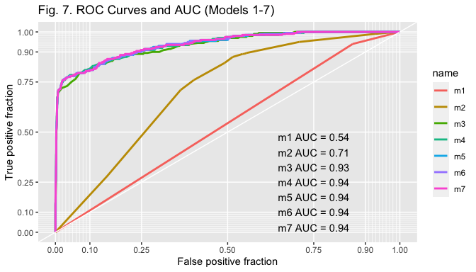
As displayed in Table 2, however, models 4 and 5 exhibit the lowest AIC score and thus seem to fit the data better, with the one of model 4 being slightly smaller. Results of the LR test confirm that the more parsimonious model 4 should be selected ( p-value > 0.05, hence the null hypothesis that the more parsimonious model is better cannot be rejected).
library(lmtest)
lrtest(m4, m5)

## Likelihood ratio test
##
## Model 1: elected ~ nameorigin + gender + agecat + ballotposition + incumbent +
##     precumulation + Left
## Model 2: elected ~ nameorigin + gender + agecat + ballotposition + incumbent +
##     precumulation + Left + foreign2018
##   #Df  LogLik Df  Chisq Pr(>Chisq)
## 1   9 -354.24
## 2  10 -353.33  1 1.8178     0.1776
4.3 Diagnostics
The GVIFs do not indicate a problem of multicollinearity (no score > 4). An outlier test reveals the presence of 232 outliers for the continuous predictor ballotposition. All these outliers however originate in the Canton of Zurich (as more seats equal ballots including more names); removing them would require eliminating all candidates at the bottom of the lists in the Canton of Zurich. In conclusion it will be explained how to better account for this problem in the future.
library(car)
vif(m4)

##                    GVIF Df GVIF^(1/(2*Df))
## nameorigin     1.035434  1        1.017563
## gender         1.148775  1        1.071809
## agecat         1.158796  2        1.037533
## ballotposition 1.052387  1        1.025859
## incumbent      1.285800  1        1.133931
## precumulation  1.023246  1        1.011556
## Left           1.162062  1        1.077990

boxplot(elections2$ballotposition, plot=FALSE)$out

##   [1] 30 33 30 27 28 28 29 34 28 32 29 26 33 32 33 31 31 28 30 30 34 29 34 34 34
##  [26] 31 31 30 26 32 26 27 31 31 27 29 29 28 31 26 33 35 29 33 28 33 27 27 26 26
##  [51] 32 35 31 26 33 32 27 26 33 30 32 29 34 35 31 32 32 27 28 31 26 26 29 34 27
##  [76] 35 28 33 29 35 33 27 35 35 33 28 26 27 34 32 35 34 28 33 26 33 29 26 29 34
## [101] 33 27 30 32 30 27 32 28 30 34 26 28 31 32 27 31 35 34 33 34 30 26 30 31 32
## [126] 34 30 30 34 34 27 29 27 34 33 35 35 33 28 34 29 30 32 30 32 33 26 29 26 33
## [151] 29 30 29 29 31 34 34 31 35 31 29 30 33 32 35 35 29 32 31 29 28 27 30 27 26
## [176] 26 34 35 31 29 35 26 31 32 26 32 35 31 26 27 33 28 27 28 29 30 31 34 32 31
## [201] 35 32 34 28 30 30 29 27 28 30 27 28 33 31 27 26 28 31 32 30 28 34 35 26 27
## [226] 32 31 31 30 33 29 26 32 33 28 28 28 35 28 33 35 32 35 27 28 27 30 29 32 35
## [251] 26 33 30 34 27 29
4.4 Results
tab_model(m4, show.loglik = T, show.aic = T, show.r2 = F, title="Table 3 - Model 4, Logistic Regression Results")
| elected | |||
|---|---|---|---|
| Predictors | Odds Ratios | CI | p |
| (Intercept) | 0.01 | 0.01 – 0.02 | <0.001 |
| nameorigin \[Non-Swiss\] | 0.34 | 0.13 – 0.78 | 0.019 |
| gender \[F\] | 1.60 | 1.01 – 2.57 | 0.048 |
| agecat \[36-60\] | 4.24 | 2.41 – 7.85 | <0.001 |
| agecat \[61+\] | 1.25 | 0.55 – 2.79 | 0.591 |
| ballotposition | 0.84 | 0.78 – 0.89 | <0.001 |
| incumbent \[1\] | 185.18 | 108.85 – 328.50 | <0.001 |
| precumulation \[1\] | 0.51 | 0.18 – 1.23 | 0.168 |
| Left \[left\] | 2.53 | 1.56 – 4.12 | <0.001 |
| Observations | 4664 | ||
| AIC | 726.477 | ||
| log-Likelihood | -354.238 | ||
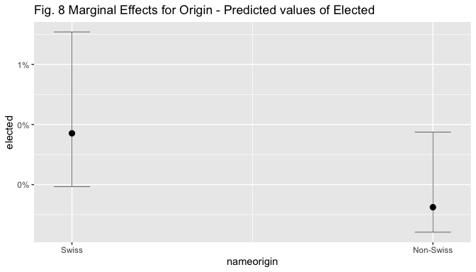
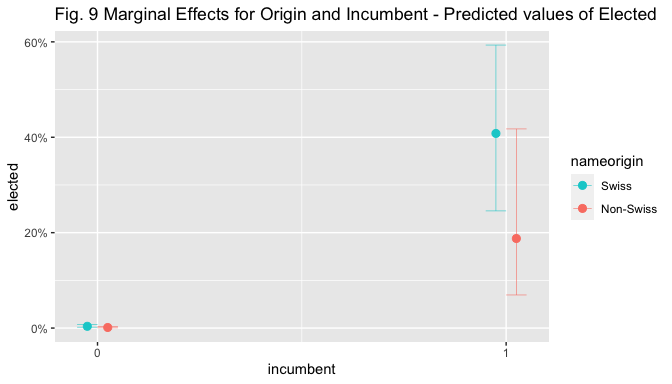
The figures below display marginal effect (ME) plots for name origin alone, name origin and incumbent (given the strong effect of incumbency found in the models), and for name origin and left (given the interest in the theoretical relation between the two).
plot_model(m4, type = "pred", line.size=0.2,
     terms = c("nameorigin"),
     colors = c("darkturquoise"),
     title = "Fig. 8 Marginal Effects for Origin - Predicted values of Elected")
plot_model(m4, type = "pred", line.size=0.2,
     terms = c("incumbent", "nameorigin"),
     colors = c("darkturquoise","salmon"),
     title = "Fig. 9 Marginal Effects for Origin and Incumbent - Predicted values of Elected ")
plot_model(m4, type = "pred", line.size=0.2,
     terms = c("Left", "nameorigin"),
     colors = c("darkturquoise","salmon"),
     title = "Fig. 10 Marginal Effects for Origin and Left - Predicted values of Elected ")
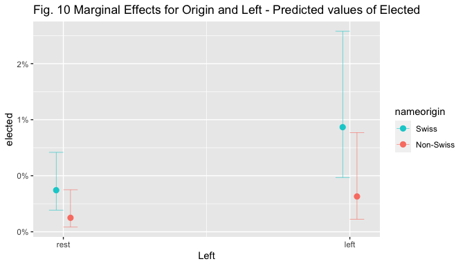
Visual inspection of the marginal effect plot for nameorigin shows that the predicted value of election goes from around 0.4% for non-Swiss to 1.1% for Swiss candidates, holding other covariates at means. The predicted values of election are similar and below 5% for both Swiss and Non-Swiss non.incumbent candidates, but when the candidate is an incumbent, the predicted value of election increases to 71% for Swiss candidates while only to 46% for non-Swiss ones, holding other covariates at means. The predicted values of election are below 0.5% for non-Swiss, non-Left-wing candidates, while they are situated above 1% for Swiss ones; they increase to 1.6% for left-wing non-Swiss candidates and to 2.4% for left-wing Swiss ones, holding other covariates at means.
4.5 Robustness Checks:
m8<- glm(elected ~ nameoriginl + gender + agecat + ballotposition + incumbent + precumulation + Left, data=elections1,
                 family=binomial(link="logit"))

m9<- glm(elected ~ nameoriginw + gender + agecat + ballotposition + incumbent + precumulation + Left, data=elections1,
                 family=binomial(link="logit"))

tab_model(m8, show.aic = TRUE, show.loglik = T, show.r2 = F, title="Table 5 - Robustness Check 1")
| elected | |||
|---|---|---|---|
| Predictors | Odds Ratios | CI | p |
| (Intercept) | 0.01 | 0.01 – 0.02 | <0.001 |
| nameoriginl \[OtherLang\] | 0.15 | 0.03 – 0.58 | 0.013 |
| nameoriginl \[SameLang\] | 0.62 | 0.18 – 1.65 | 0.387 |
| gender \[F\] | 1.58 | 1.00 – 2.55 | 0.054 |
| agecat \[36-60\] | 4.18 | 2.37 – 7.74 | <0.001 |
| agecat \[61+\] | 1.20 | 0.53 – 2.69 | 0.662 |
| ballotposition | 0.84 | 0.78 – 0.89 | <0.001 |
| incumbent | 190.83 | 111.50 – 341.24 | <0.001 |
| precumulation | 0.51 | 0.18 – 1.23 | 0.169 |
| Left \[left\] | 2.61 | 1.60 – 4.26 | <0.001 |
| Observations | 4664 | ||
| AIC | 726.073 | ||
| log-Likelihood | -353.037 | ||
| elected | |||
|---|---|---|---|
| Predictors | Odds Ratios | CI | p |
| (Intercept) | 0.01 | 0.01 – 0.02 | <0.001 |
| nameoriginw \[non-Western\] | 0.26 | 0.05 – 0.99 | 0.085 |
| nameoriginw \[Western\] | 0.39 | 0.12 – 1.05 | 0.090 |
| gender \[F\] | 1.60 | 1.01 – 2.57 | 0.049 |
| agecat \[36-60\] | 4.22 | 2.39 – 7.81 | <0.001 |
| agecat \[61+\] | 1.24 | 0.54 – 2.77 | 0.609 |
| ballotposition | 0.84 | 0.78 – 0.89 | <0.001 |
| incumbent | 185.88 | 109.16 – 330.17 | <0.001 |
| precumulation | 0.51 | 0.18 – 1.23 | 0.167 |
| Left \[left\] | 2.55 | 1.56 – 4.15 | <0.001 |
| Observations | 4664 | ||
| AIC | 728.304 | ||
| log-Likelihood | -354.152 | ||
5. Conclusion
To conclude, results of the statistical analyses suggest that bearing a non-Swiss name exerts a negative effect on the chances of being elected, and this even after controlling for multiple individual characteristics of candidates that may affect their electoral success. The local-level findings of Portmann and Stojanović (2019) find support in this federal level assessment. Further studies and a better model specification are however needed to draw conclusions. Three main limitations should in fact be addressed. First, the use of a binary dependent variable to measure electoral success may conceal important information and variation that would instead be visible by using a continuous measure such as vote share. However, computing vote share is not a simple task due to the complex PR system that involves the possibility of casting preferences within and across lists; moreover, the unequal number of votes casted per electoral district should also be taken into account. Future studies should however consider the use of such a measure. Second, the structure of Swiss election data would require to be taken into account through a multi-level model allowing to take into account the nestedness of individuals within party lists and cantons. Finally, a minor limitation regards the way in which ballot position has been measured. To account for cantonal differences in ballot size position could have been measured in percentiles, instead absolute numbers. The six cantons electing only one seat using the majoritarian system should instead be removed or considered as missing as their candidates are necessarily on top of the lists. In spite of these limitations, this project suggests that electoral discrimination in Switzerland is a topic (and possibly a problem) worth further investigation.
References
Black, Jerome and Lynda Erickson. 2006. “Ethno-racial Origins of Candidates and Electoral Performance.” Party Politics 12(4): 541-561.
Bloemraad, Irene and Karen Schönwälder. 2013. “Immigrant and Ethnic Minority Representation in Europe: Conceptual Challenges and Theoretical Approaches.” West European Politics 36(3): 564-579.
Fibbi, Rosita, Mathias Lerch and Philipp Wanner. 2007. “Naturalisation and Socio-Economic Characteristics of Youth of Immigrant Descent in Switzerland.” Journal of Ethnic and Migration Studies 33(7): 1121-1144.
McDermott, Monika. 1998. “Race and gender cues in low-information elections.” Political Research Quarterly 51(4): 895-918.
Nguyen, Duc-Quang. 2016. “244 millions d’immigrés dans le monde, quel pays en dénombre le plus?” Swissinfo, 13 September 2016 https://www.swissinfo.ch/fre/s%C3%A9rie-migration-partie-2-_244-millions-d-immigr%C3%A9s-dans-le-monde-quel-pays-en-d%C3%A9nombre-le-plus/42392104
OFS. 2019a. Population résidante permanente selon le sexe, le lieu de naissance, la durée de résidence, la catégorie de nationalité et l’autorisation de résidence, 2010-2018. Available at: https://www.bfs.admin.ch/bfs/fr/home/statistiques/population/migration-integration/selon-lieu-naissance.html
OFS. 2019b. “Population selon le statut migratoire.” Office fédéral de la Statistique - Migration et Intégration. Last Accessed on May 25, 2020. https://www.bfs.admin.ch/bfs/fr/home/statistiques/population/migration-integration/selon-statut-migratoire.html
OFS. 2020. “Population résidante permanente étrangère, en 2018.” Atlas statistique de la Suisse. https://www.atlas.bfs.admin.ch/maps/13/fr/14472_90_89_70/23060.html
Opendata.swiss. 2019. “Elections Fédérales 2019 - CN - Candidats (Canton) (INT2).” Dataset available at: https://opendata.swiss/fr/dataset/eidg-wahlen-2019/resource/8df0f8b2-f213-47b1-b714-b7bff03fc229
Portmann Lea and Nenad Stojanović. 2019. “Electoral Discrimination Against Immigrant-Origin Candidates.” Political Behavior41(1):105-134.
RSS. 2020. “The Register of Swiss Surnames.” Historical Dictionary of Switzerland. https://hls-dhs-dss.ch/famn/index.php?lg=e
Street, Alex. 2014. “Representation Despite Discrimination: Minority Candidates in Germany.” Political Research Quarterly 67(2): 374-385.
Thrasher, Michael et al. 2015. “Candidate Ethnic Origins and Voter Preferences: Examining Name Discrimination in Local Elections in Britain.” British Journal of Political Science 47:413-435.
Co-Director
Global Governance Centre
Professor
International Relations and Political Science
President
Global Governance Research Centre Consortium
International institutions and political networks.