Augusta Nannerini

Last updated on 18 Feb, 2021 27 min read

1. Introduction
2. Data
3. Methods
4. Results
5. Conclusion
References:

1. Introduction

The question that my research aims at asking is whether having a national ID (coded by the variable fin48) has an impact on the possibility for people to be part of the workforce in Jordan. The interest in the issue came from the fact that Jordan hosts one of the largest population of forced displaced people in the world, the majority of them without official documentations. (ODI, 2019; Fallah, Krafft, Wahba, 2019). The research question that this analysis seeks to answer is therefore the following: “Does having a national ID has an impact on the possibility to be part of the workforce in Jordan?”

2. Data

We work with a World Bank Dataset called “Global Findex”, which reports data about the level of access to formal and informal ways of savings, as well as employment. Our dependent variable will be “emp_in”, indicating the possibility for the respondent to be part of the workforce. Crucially, this variable captures both employment in the formal and in the informal labour market.For this purpose, in our first model we will use the variable that indicates if the respondent has a national ID as a main explanatory, controlling for gender (female) and age. In our second model, to test an alternative hypothesis, we will use as explanatory variable the level of education, and we will control for the other variables listed above (including fin48). In the third model we will add control variables for the possibility to save to start a business (fin15) and possibility to save for old age (fin16). Fin15 and Fin16 are interesting variables to build up my theory, as they provide additional information regarding the conditions and preferences of the labour forced in the Jordanian labour market. With the exception of the variable for age, all the others are categorical variables with binomial responses.

—PREPARING THE DATASET AND VISUALISE THE DISTRIBUTION OF THE VARIABLES———-

#Import the dataset

library(haven)
 micro_world <- read_dta("micro_world.dta")
View(micro_world)

We see that in this dataset there are 154923 observations and 105 variables. This high number is explained by the fact that the dataset collects observations from countries all over the world. We will limit our study to the country of Jordan.

#Modify the dataset in order to have data only about Jordan

library(tidyverse)

## ── Attaching packages ────────────────────────────────────────────────────────────────────────────────────────────────── tidyverse 1.3.0 ──

## ✓ ggplot2 3.3.0     ✓ purrr   0.3.4
## ✓ tibble  3.0.1     ✓ dplyr   0.8.5
## ✓ tidyr   1.0.2     ✓ stringr 1.4.0
## ✓ readr   1.3.1     ✓ forcats 0.5.0

## ── Conflicts ───────────────────────────────────────────────────────────────────────────────────────────────────── tidyverse_conflicts() ──
## x dplyr::filter() masks stats::filter()
## x dplyr::lag()    masks stats::lag()

newdata <- filter (micro_world, economy == "Jordan")
View(newdata)
summary(newdata)

##    economy          economycode          regionwb           pop_adult      
##  Length:1012        Length:1012        Length:1012        Min.   :6072449  
##  Class :character   Class :character   Class :character   1st Qu.:6072449  
##  Mode  :character   Mode  :character   Mode  :character   Median :6072449  
##                                                           Mean   :6072449  
##                                                           3rd Qu.:6072449  
##                                                           Max.   :6072449  
##                                                                            
##   wpid_random             wgt             female           age       
##  Min.   :111128048   Min.   :0.2918   Min.   :1.000   Min.   :15.00  
##  1st Qu.:133968623   1st Qu.:0.5788   1st Qu.:1.000   1st Qu.:24.00  
##  Median :160477715   Median :0.8683   Median :2.000   Median :34.00  
##  Mean   :160313166   Mean   :1.0000   Mean   :1.597   Mean   :37.07  
##  3rd Qu.:184710130   3rd Qu.:1.3156   3rd Qu.:2.000   3rd Qu.:47.00  
##  Max.   :210982185   Max.   :2.6549   Max.   :2.000   Max.   :99.00  
##                                                                      
##       educ           inc_q           emp_in            fin2     
##  Min.   :1.000   Min.   :1.000   Min.   :0.0000   Min.   :1.00  
##  1st Qu.:1.000   1st Qu.:2.000   1st Qu.:0.0000   1st Qu.:1.00  
##  Median :2.000   Median :3.000   Median :0.0000   Median :2.00  
##  Mean   :1.886   Mean   :3.154   Mean   :0.3864   Mean   :1.71  
##  3rd Qu.:2.000   3rd Qu.:4.000   3rd Qu.:1.0000   3rd Qu.:2.00  
##  Max.   :4.000   Max.   :5.000   Max.   :1.0000   Max.   :3.00  
##                                                                 
##       fin3            fin4           fin5            fin6            fin7      
##  Min.   :1.000   Min.   :1.00   Min.   :1.000   Min.   :1.000   Min.   :1.000  
##  1st Qu.:1.000   1st Qu.:1.00   1st Qu.:2.000   1st Qu.:1.000   1st Qu.:2.000  
##  Median :1.000   Median :2.00   Median :2.000   Median :2.000   Median :2.000  
##  Mean   :1.033   Mean   :1.73   Mean   :1.901   Mean   :1.734   Mean   :1.986  
##  3rd Qu.:1.000   3rd Qu.:2.00   3rd Qu.:2.000   3rd Qu.:2.000   3rd Qu.:2.000  
##  Max.   :2.000   Max.   :2.00   Max.   :2.000   Max.   :2.000   Max.   :3.000  
##  NA's   :710     NA's   :720    NA's   :647     NA's   :647                    
##       fin8            fin9           fin10           fin11a     
##  Min.   :1.000   Min.   :1.000   Min.   :1.000   Min.   :1.000  
##  1st Qu.:1.000   1st Qu.:1.000   1st Qu.:1.000   1st Qu.:2.000  
##  Median :1.000   Median :1.000   Median :1.000   Median :2.000  
##  Mean   :1.308   Mean   :1.219   Mean   :1.192   Mean   :1.966  
##  3rd Qu.:2.000   3rd Qu.:1.000   3rd Qu.:1.000   3rd Qu.:2.000  
##  Max.   :2.000   Max.   :2.000   Max.   :2.000   Max.   :3.000  
##  NA's   :986     NA's   :642     NA's   :642     NA's   :370    
##      fin11b          fin11c          fin11d          fin11e     
##  Min.   :1.000   Min.   :1.000   Min.   :1.000   Min.   :1.000  
##  1st Qu.:1.000   1st Qu.:2.000   1st Qu.:2.000   1st Qu.:2.000  
##  Median :2.000   Median :2.000   Median :2.000   Median :2.000  
##  Mean   :1.681   Mean   :1.905   Mean   :1.885   Mean   :1.849  
##  3rd Qu.:2.000   3rd Qu.:2.000   3rd Qu.:2.000   3rd Qu.:2.000  
##  Max.   :3.000   Max.   :3.000   Max.   :3.000   Max.   :3.000  
##  NA's   :370     NA's   :370     NA's   :370     NA's   :370    
##      fin11f          fin11g          fin11h          fin14a         fin14b     
##  Min.   :1.000   Min.   :1.000   Min.   :1.000   Min.   :1.00   Min.   :1.000  
##  1st Qu.:1.000   1st Qu.:1.000   1st Qu.:1.000   1st Qu.:2.00   1st Qu.:2.000  
##  Median :1.000   Median :2.000   Median :2.000   Median :2.00   Median :2.000  
##  Mean   :1.249   Mean   :1.737   Mean   :1.586   Mean   :1.99   Mean   :1.939  
##  3rd Qu.:1.000   3rd Qu.:2.000   3rd Qu.:2.000   3rd Qu.:2.00   3rd Qu.:2.000  
##  Max.   :3.000   Max.   :3.000   Max.   :3.000   Max.   :3.00   Max.   :3.000  
##  NA's   :370     NA's   :370     NA's   :370                                   
##      fin14c          fin15           fin16           fin17a     
##  Min.   :1.000   Min.   :1.000   Min.   :1.000   Min.   :1.000  
##  1st Qu.:1.000   1st Qu.:2.000   1st Qu.:2.000   1st Qu.:2.000  
##  Median :2.000   Median :2.000   Median :2.000   Median :2.000  
##  Mean   :1.712   Mean   :1.939   Mean   :1.898   Mean   :1.909  
##  3rd Qu.:2.000   3rd Qu.:2.000   3rd Qu.:2.000   3rd Qu.:2.000  
##  Max.   :2.000   Max.   :3.000   Max.   :3.000   Max.   :3.000  
##  NA's   :939                                                    
##      fin17b          fin19           fin20           fin21      
##  Min.   :1.000   Min.   :1.000   Min.   :1.000   Min.   :1.000  
##  1st Qu.:2.000   1st Qu.:2.000   1st Qu.:2.000   1st Qu.:2.000  
##  Median :2.000   Median :2.000   Median :2.000   Median :2.000  
##  Mean   :1.807   Mean   :1.874   Mean   :1.903   Mean   :1.973  
##  3rd Qu.:2.000   3rd Qu.:2.000   3rd Qu.:2.000   3rd Qu.:2.000  
##  Max.   :3.000   Max.   :3.000   Max.   :3.000   Max.   :3.000  
##                                                                 
##      fin22a          fin22b          fin22c          fin24           fin25     
##  Min.   :1.000   Min.   :1.000   Min.   :1.000   Min.   :1.000   Min.   :1.00  
##  1st Qu.:2.000   1st Qu.:1.000   1st Qu.:1.000   1st Qu.:1.000   1st Qu.:2.00  
##  Median :2.000   Median :2.000   Median :2.000   Median :1.000   Median :2.00  
##  Mean   :1.844   Mean   :1.696   Mean   :1.693   Mean   :1.375   Mean   :2.12  
##  3rd Qu.:2.000   3rd Qu.:2.000   3rd Qu.:2.000   3rd Qu.:2.000   3rd Qu.:2.00  
##  Max.   :3.000   Max.   :3.000   Max.   :4.000   Max.   :3.000   Max.   :6.00  
##                                  NA's   :807                     NA's   :362   
##      fin26           fin27a          fin27b       fin27c1         fin27c2     
##  Min.   :1.000   Min.   :1.000   Min.   :1     Min.   :1.000   Min.   :1.000  
##  1st Qu.:2.000   1st Qu.:2.000   1st Qu.:2     1st Qu.:1.000   1st Qu.:2.000  
##  Median :2.000   Median :2.000   Median :2     Median :1.000   Median :2.000  
##  Mean   :1.878   Mean   :1.828   Mean   :2     Mean   :1.136   Mean   :1.873  
##  3rd Qu.:2.000   3rd Qu.:2.000   3rd Qu.:2     3rd Qu.:1.000   3rd Qu.:2.000  
##  Max.   :3.000   Max.   :3.000   Max.   :3     Max.   :2.000   Max.   :2.000  
##                  NA's   :878     NA's   :878   NA's   :902     NA's   :902    
##      fin28           fin29a          fin29b         fin29c1     
##  Min.   :1.000   Min.   :1.000   Min.   :2.000   Min.   :1.000  
##  1st Qu.:2.000   1st Qu.:2.000   1st Qu.:2.000   1st Qu.:1.000  
##  Median :2.000   Median :2.000   Median :2.000   Median :1.000  
##  Mean   :1.835   Mean   :1.888   Mean   :2.006   Mean   :1.108  
##  3rd Qu.:2.000   3rd Qu.:2.000   3rd Qu.:2.000   3rd Qu.:1.000  
##  Max.   :3.000   Max.   :3.000   Max.   :3.000   Max.   :2.000  
##                  NA's   :833     NA's   :833     NA's   :854    
##     fin29c2          fin30          fin31a          fin31b          fin31c     
##  Min.   :1.000   Min.   :1.00   Min.   :1.000   Min.   :1.000   Min.   :1.000  
##  1st Qu.:2.000   1st Qu.:1.00   1st Qu.:2.000   1st Qu.:2.000   1st Qu.:1.000  
##  Median :2.000   Median :2.00   Median :2.000   Median :2.000   Median :1.000  
##  Mean   :1.918   Mean   :1.61   Mean   :1.909   Mean   :1.993   Mean   :1.022  
##  3rd Qu.:2.000   3rd Qu.:2.00   3rd Qu.:2.000   3rd Qu.:2.000   3rd Qu.:1.000  
##  Max.   :3.000   Max.   :3.00   Max.   :2.000   Max.   :2.000   Max.   :3.000  
##  NA's   :854                    NA's   :605     NA's   :605     NA's   :644    
##      fin32           fin33           fin34a          fin34b         fin34c1    
##  Min.   :1.000   Min.   :1.000   Min.   :1.000   Min.   :1.000   Min.   :1.00  
##  1st Qu.:2.000   1st Qu.:1.000   1st Qu.:1.000   1st Qu.:2.000   1st Qu.:1.00  
##  Median :2.000   Median :2.000   Median :2.000   Median :2.000   Median :1.00  
##  Mean   :1.796   Mean   :1.688   Mean   :1.512   Mean   :1.991   Mean   :1.11  
##  3rd Qu.:2.000   3rd Qu.:2.000   3rd Qu.:2.000   3rd Qu.:2.000   3rd Qu.:1.00  
##  Max.   :3.000   Max.   :3.000   Max.   :2.000   Max.   :2.000   Max.   :2.00  
##                  NA's   :797     NA's   :797     NA's   :797     NA's   :903   
##     fin34c2        fin35           fin36           fin37           fin38     
##  Min.   :2     Min.   :1.000   Min.   :1.000   Min.   :1.000   Min.   :1.00  
##  1st Qu.:2     1st Qu.:1.000   1st Qu.:1.000   1st Qu.:2.000   1st Qu.:2.00  
##  Median :2     Median :1.000   Median :1.000   Median :2.000   Median :2.00  
##  Mean   :2     Mean   :1.425   Mean   :1.066   Mean   :1.922   Mean   :1.88  
##  3rd Qu.:2     3rd Qu.:2.000   3rd Qu.:1.000   3rd Qu.:2.000   3rd Qu.:2.00  
##  Max.   :2     Max.   :2.000   Max.   :2.000   Max.   :3.000   Max.   :3.00  
##  NA's   :903   NA's   :906     NA's   :951                                   
##      fin39a         fin39b       fin39c1        fin39c2          fin40      
##  Min.   :1.00   Min.   :2     Min.   :1.00   Min.   :1.000   Min.   :1.000  
##  1st Qu.:1.00   1st Qu.:2     1st Qu.:1.00   1st Qu.:2.000   1st Qu.:1.000  
##  Median :1.00   Median :2     Median :2.00   Median :2.000   Median :1.000  
##  Mean   :1.21   Mean   :2     Mean   :1.61   Mean   :1.878   Mean   :1.273  
##  3rd Qu.:1.00   3rd Qu.:2     3rd Qu.:2.00   3rd Qu.:2.000   3rd Qu.:1.750  
##  Max.   :2.00   Max.   :2     Max.   :2.00   Max.   :2.000   Max.   :2.000  
##  NA's   :817    NA's   :817   NA's   :971    NA's   :971     NA's   :990    
##      fin41           fin42           fin43a          fin43b       fin43c1   
##  Min.   :1.000   Min.   :1.000   Min.   :1.000   Min.   :2     Min.   :1.0  
##  1st Qu.:1.000   1st Qu.:2.000   1st Qu.:2.000   1st Qu.:2     1st Qu.:1.0  
##  Median :1.000   Median :2.000   Median :2.000   Median :2     Median :1.0  
##  Mean   :1.062   Mean   :1.988   Mean   :1.909   Mean   :2     Mean   :1.1  
##  3rd Qu.:1.000   3rd Qu.:2.000   3rd Qu.:2.000   3rd Qu.:2     3rd Qu.:1.0  
##  Max.   :2.000   Max.   :3.000   Max.   :2.000   Max.   :2     Max.   :2.0  
##  NA's   :996                     NA's   :990     NA's   :990   NA's   :992  
##     fin43c2        fin44          fin45          fin46          fin47a     
##  Min.   :2     Min.   :2      Min.   : NA    Min.   :1.00   Min.   :1.000  
##  1st Qu.:2     1st Qu.:2      1st Qu.: NA    1st Qu.:2.00   1st Qu.:2.000  
##  Median :2     Median :2      Median : NA    Median :2.00   Median :2.000  
##  Mean   :2     Mean   :2      Mean   :NaN    Mean   :1.91   Mean   :1.875  
##  3rd Qu.:2     3rd Qu.:2      3rd Qu.: NA    3rd Qu.:2.00   3rd Qu.:2.000  
##  Max.   :2     Max.   :2      Max.   : NA    Max.   :3.00   Max.   :2.000  
##  NA's   :992   NA's   :1010   NA's   :1012   NA's   :232    NA's   :932    
##      fin47b         fin47c1         fin47c2       fin47c3         fin47c4   
##  Min.   :1.000   Min.   :1.000   Min.   :2     Min.   :1.000   Min.   :2    
##  1st Qu.:2.000   1st Qu.:1.000   1st Qu.:2     1st Qu.:2.000   1st Qu.:2    
##  Median :2.000   Median :1.000   Median :2     Median :2.000   Median :2    
##  Mean   :1.988   Mean   :1.014   Mean   :2     Mean   :1.978   Mean   :2    
##  3rd Qu.:2.000   3rd Qu.:1.000   3rd Qu.:2     3rd Qu.:2.000   3rd Qu.:2    
##  Max.   :2.000   Max.   :2.000   Max.   :2     Max.   :2.000   Max.   :2    
##  NA's   :932     NA's   :943     NA's   :943   NA's   :966     NA's   :966  
##     fin47c5       mobileowner        fin48        account_fin    
##  Min.   :1.000   Min.   :1.000   Min.   :1.000   Min.   :0.0000  
##  1st Qu.:2.000   1st Qu.:1.000   1st Qu.:1.000   1st Qu.:0.0000  
##  Median :2.000   Median :1.000   Median :1.000   Median :0.0000  
##  Mean   :1.978   Mean   :1.091   Mean   :1.103   Mean   :0.4101  
##  3rd Qu.:2.000   3rd Qu.:1.000   3rd Qu.:1.000   3rd Qu.:1.0000  
##  Max.   :2.000   Max.   :2.000   Max.   :3.000   Max.   :1.0000  
##  NA's   :966                                                     
##   account_mob          account          saved           borrowed     
##  Min.   :0.000000   Min.   :0.000   Min.   :0.0000   Min.   :0.0000  
##  1st Qu.:0.000000   1st Qu.:0.000   1st Qu.:0.0000   1st Qu.:0.0000  
##  Median :0.000000   Median :0.000   Median :0.0000   Median :0.0000  
##  Mean   :0.009881   Mean   :0.413   Mean   :0.4397   Mean   :0.4783  
##  3rd Qu.:0.000000   3rd Qu.:1.000   3rd Qu.:1.0000   3rd Qu.:1.0000  
##  Max.   :1.000000   Max.   :1.000   Max.   :1.0000   Max.   :1.0000  
##                                                                      
##  receive_wages   receive_transfers receive_pension receive_agriculture
##  Min.   :1.000   Min.   :1.000     Min.   :1.000   Min.   :1.000      
##  1st Qu.:4.000   1st Qu.:4.000     1st Qu.:4.000   1st Qu.:4.000      
##  Median :4.000   Median :4.000     Median :4.000   Median :4.000      
##  Mean   :3.491   Mean   :3.788     Mean   :3.642   Mean   :3.966      
##  3rd Qu.:4.000   3rd Qu.:4.000     3rd Qu.:4.000   3rd Qu.:4.000      
##  Max.   :5.000   Max.   :5.000     Max.   :5.000   Max.   :5.000      
##                                                                       
##  pay_utilities    remittances      pay_onlne       pay_onlne_mobintbuy
##  Min.   :1.000   Min.   :1.000   Min.   :0.00000   Min.   :0.0000     
##  1st Qu.:2.000   1st Qu.:3.000   1st Qu.:0.00000   1st Qu.:0.0000     
##  Median :4.000   Median :5.000   Median :0.00000   Median :0.0000     
##  Mean   :3.176   Mean   :4.413   Mean   :0.02075   Mean   :0.2877     
##  3rd Qu.:4.000   3rd Qu.:5.000   3rd Qu.:0.00000   3rd Qu.:1.0000     
##  Max.   :5.000   Max.   :6.000   Max.   :1.00000   Max.   :1.0000     
##                                                    NA's   :939        
##     pay_cash       pay_cash_mobintbuy
##  Min.   :0.00000   Min.   :0.0000    
##  1st Qu.:0.00000   1st Qu.:0.0000    
##  Median :0.00000   Median :1.0000    
##  Mean   :0.05138   Mean   :0.7123    
##  3rd Qu.:0.00000   3rd Qu.:1.0000    
##  Max.   :1.00000   Max.   :1.0000    
##                    NA's   :939

The new dataset that we obtain has 1012 observations, and still 105 variables. However, this total number of observations will be reduced by the time that we treat missing data and the variables that report “don’t know” as a response. More detail will become clearer in the next steps of the analysis.

We now check for the presence of missing data in the variables that we are going to take into account in our models

newdata2 <- newdata  
newdata2[sample(1:nrow(newdata2), 4), "emp_in"] <- NA
newdata2[sample(1:nrow(newdata2), 4), "educ"] <- NA
newdata2[sample(1:nrow(newdata2), 4), "female"] <- NA
newdata2[sample(1:nrow(newdata2), 4), "fin15"] <- NA
newdata2[sample(1:nrow(newdata2), 4), "fin16"] <- NA
newdata2[sample(1:nrow(newdata2), 4), "fin48"] <- NA
newdata2[sample(1:nrow(newdata2), 4), "age"] <- NA
library(Amelia)

## Loading required package: Rcpp

## ## 
## ## Amelia II: Multiple Imputation
## ## (Version 1.7.6, built: 2019-11-24)
## ## Copyright (C) 2005-2020 James Honaker, Gary King and Matthew Blackwell
## ## Refer to http://gking.harvard.edu/amelia/ for more information
## ##

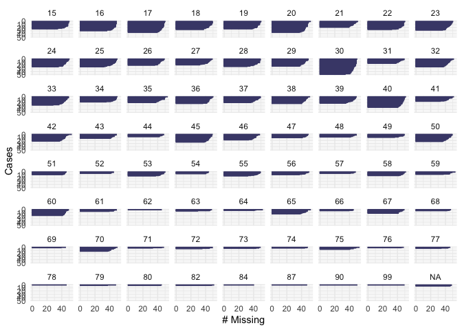
missmap(newdata2)

## Warning: Unknown or uninitialised column: `arguments`.

## Warning: Unknown or uninitialised column: `arguments`.

## Warning: Unknown or uninitialised column: `imputations`.

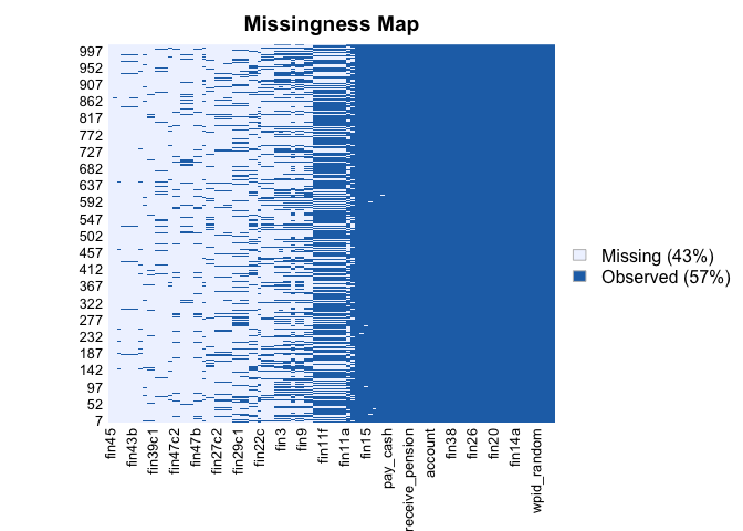Usig the package “Amelia” we see that there is a high number of missing data (43%). Luckily, the fact the we are using a very large dataset means that even if we reduce 43% of the size of the data, we don’t completely reduce the statistical power of the model. Given that nature of the data and the World Bank Description about how they were gathered, we assume that this data are “MACR”, Missing Completely At Random.

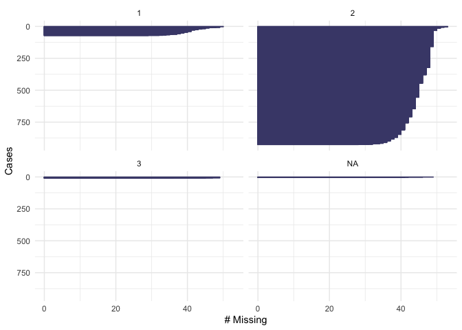
We now want to check if the missing data are in our variables of interests and in which percentage, and we do so by building a plot that will also help us to see the distribution of our variables of interest

library(naniar)
gg_miss_case(newdata2, emp_in, order_cases = TRUE, show_pct = FALSE)

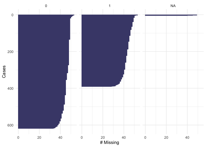
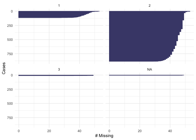
gg_miss_case(newdata2, educ, order_cases = TRUE, show_pct = FALSE)

gg_miss_case(newdata2, female, order_cases = TRUE, show_pct = FALSE)

gg_miss_case(newdata2, age, order_cases = TRUE, show_pct = FALSE)

gg_miss_case(newdata2, fin15, order_cases = TRUE, show_pct = FALSE)

gg_miss_case(newdata2, fin16, order_cases = TRUE, show_pct = FALSE)

fct_explicit_na("fin48", na_level = "(Missing)")

## [1] fin48
## Levels: fin48

gg_miss_case(newdata2, fin48, order_cases = TRUE, show_pct = FALSE)

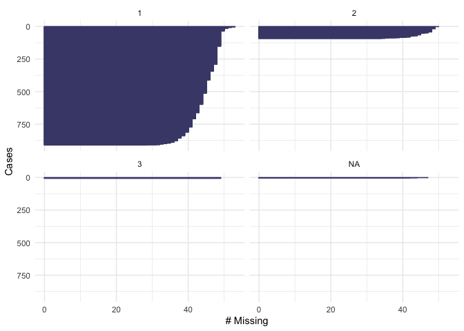
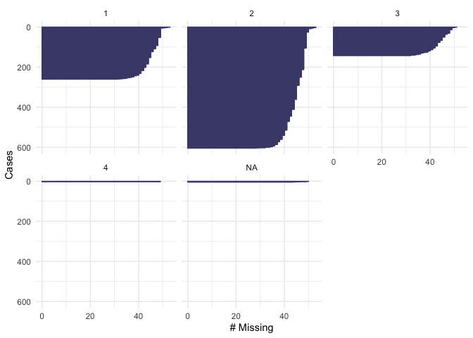
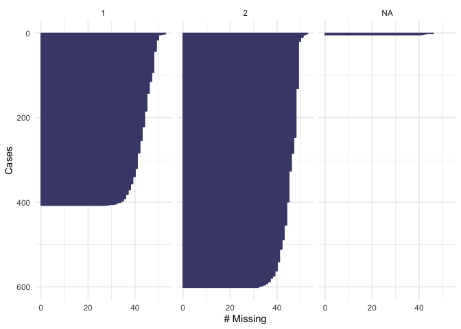
From the plot we see that our dependent variable, being part of the workforce, doesn’t have missing values. We also note that 600 respondents are out of the workforce and 400 are in the workforce. Looking at education, we see that there are not missing values. About 200 respondents have “level 1” of education, 600 have “level 2” and 150 have “level 3”. None of the respondents have “level 4”. In the variable “female”, there are not missing values. 400 of the respondents were men and 600 were female. For the variable of “age” we see that there are not missing values and that the majority of the respondents were below age 50. In the variable fin15 (having saved to start a business) there is a small number of missing data (>50). More than 800 respondents reported not to have saved, and about 100 reported to have saved to start a business. In the variable fin16 (having saved for old age), there is a small number of missing data (>50). More than 800 respondents reported not to have saved, and only about 150 reported to have saved. In the case of fin48 (having a national ID), there is a small number of missing data (>50). More than 850 respondents reported to have a national ID, and only about 100 respondents reported not to have a national ID. Because these numbers are low compared to the total number of observations that we have in the dataset, we will omit them when running our model

#We now look at our categorical variables. We use table()function to find the distribution of categorical variables and pay attention to the “don’t know” values

library(table1)

## 
## Attaching package: 'table1'

## The following objects are masked from 'package:base':
## 
##     units, units<-

table(newdata2$fin15)

## 
##   1   2   3 
##  72 926  10

table(newdata2$fin48)

## 
##   1   2   3 
## 910  92   6

table(newdata2$female)

## 
##   1   2 
## 407 601

table(newdata2$fin16)

## 
##   1   2   3 
## 114 884  10

table(newdata2$emp_in)

## 
##   0   1 
## 618 390

We see that the variables fin15(saved for business purpose), fin48 (having a national ID) and fin16 (saved for old age) have a small number of “dk” responses

#We find the percentage distribution of these “dk” values to see how much they matter in the overall dataset

table(newdata2$fin15)/nrow(newdata2)

## 
##           1           2           3 
## 0.071146245 0.915019763 0.009881423

table(newdata2$fin48)/nrow(newdata2)

## 
##           1           2           3 
## 0.899209486 0.090909091 0.005928854

table(newdata2$fin16)/nrow(newdata2)

## 
##           1           2           3 
## 0.112648221 0.873517787 0.009881423

It is confirmed that the “dk” answers are in a very limited number and we can therefore treat them as missing values. This means that the total number of observations that will be used in the model is less than the total number presented in the dataset

#We now treat as “factors” the categorical variables and then treat the “dk” as NA

library(pscl)

## Classes and Methods for R developed in the
## Political Science Computational Laboratory
## Department of Political Science
## Stanford University
## Simon Jackman
## hurdle and zeroinfl functions by Achim Zeileis

library(tidyverse)
library(pscl)
newdata2 <- newdata2 %>%
mutate(female = as_factor(female), fin15 = as_factor(fin15), fin48 = as_factor(fin48), fin16 = as_factor(fin16) , emp_in = as_factor(emp_in))
library(forcats)
anyNA(fct_drop(newdata2$fin48, only = "(dk)"))

## [1] TRUE

newdata2$fin48[newdata2$fin48=="(dk)"]<-NA
sum(is.na(newdata2$fin48)*1)

## [1] 10

anyNA(fct_drop(newdata2$fin16, only = "(dk)"))

## [1] TRUE

newdata2$fin16[newdata2$fin16=="(dk)"]<-NA
sum(is.na(newdata2$fin16)*1)

## [1] 14

anyNA(fct_drop(newdata2$fin15, only = "(dk)"))

## [1] TRUE

newdata2$fin15[newdata2$fin15=="(dk)"]<-NA
sum(is.na(newdata2$fin15)*1)

## [1] 14

Now our dataset is ready to be analysed.

3. Methods

Given that we are working with categorical variables, and that our dependent variable has a binomial response (yes/no), we run a logistic regression for binomial models (gml) ————MODELLING——————– #MOD1: As explained in the introduction, Mod1 has per DV if the respondent is in the workforce, and the main explanatory variable is fin48 (having or not a national ID). Control for gender and age

mod1 <- glm(emp_in ~ fin48 + female + age, 
            data=newdata2, 
            family=binomial(link="logit"))
library(sjPlot)
tab_model(mod1)

	Respondent is in the workforce
Predictors	Odds Ratios	CI	p
(Intercept)	5.07	3.28 – 7.97	<0.001
fin48: no	0.39	0.22 – 0.67	0.001
Respondent is female: Female	0.11	0.08 – 0.15	<0.001
Respondent age	0.98	0.97 – 0.99	<0.001
Observations	990
R² Tjur	0.254

Interpretation: We build a table that allows us to look at the odds ratio. This means that coefficents with values above 1 increase the odds, while values below 1 decrease the odds of being in the work force. Remarkably, all the p values in the table are less than 0.005. National ID has a coefficient of 0.39 and p value of 0.001, which means that it decreases the odds of being in the workforce. The variable for gender has a very small p value, <0.001 with coefficient of 0.12. This means that being a woman decreases the odds of being in the workforce. Age has a p value of <0.001 and coefficient 0.98, meaning that it decreases the odds of being in the workforce.

————CHECKS MOD1——————– First, we check for multicollinearity

library(car)

## Loading required package: carData

## Registered S3 methods overwritten by 'car':
##   method                          from
##   influence.merMod                lme4
##   cooks.distance.influence.merMod lme4
##   dfbeta.influence.merMod         lme4
##   dfbetas.influence.merMod        lme4

## 
## Attaching package: 'car'

## The following object is masked from 'package:dplyr':
## 
##     recode

## The following object is masked from 'package:purrr':
## 
##     some

t(t(vif(mod1)))

##            [,1]
## fin48  1.099499
## female 1.024280
## age    1.093507

It’s assumed that there is collinearity among the variables if the coefficient is > 4. Luckily, we don’t find collinearity in the model

We can also check visually

library(performance)
plot(check_collinearity(mod1))

we confirm that there is not multicollinearity

We now look at the residuals

mod1 <- glm(emp_in ~ fin48 + female +age, 
            data=newdata2, family = "binomial")
binned_residuals(mod1)

## Warning: Probably bad model fit. Only about 61% of the residuals are inside the error bounds.

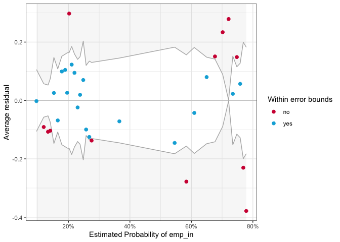It seems that the majority of the residuals fell outside the “error bound”, which indicates that there is a problem in our model

We now test for heteroskedasticity. We run Breush-Pagan test, where the null hypothesis is that there is not heteroskedasticity.

library(lmtest)

## Loading required package: zoo

## 
## Attaching package: 'zoo'

## The following objects are masked from 'package:base':
## 
##     as.Date, as.Date.numeric

bptest(mod1, data = newdata2, studentize = TRUE)

## 
##  studentized Breusch-Pagan test
## 
## data:  mod1
## BP = 19.496, df = 3, p-value = 0.0002158

P value is >0.05. Hence, we fail to reject the null hypothesis of homogeneity and we accept that there is heteroskedasticity in the model

We treat heteroskedasticity by clustering by the variable age

library(sandwich)
tab_model(mod1, vcov.fun = "CL", vcov.args = ~ age, show.obs = F, show.r2 = F, show.se = T, show.stat = T)

	Respondent is in the workforce
Predictors	Odds Ratios	std. Error	CI	Statistic	p
(Intercept)	5.07	0.43	2.17 – 11.87	3.75	<0.001
fin48: no	0.39	0.61	0.12 – 1.27	-1.57	0.117
Respondent is female: Female	0.11	0.16	0.08 – 0.15	-14.13	<0.001
Respondent age	0.98	0.01	0.96 – 1.00	-2.36	0.019

Interpretation: Once we cluster mod1 by age, we see that fin48 is not statistically significant anymore. However, being a woman still decreases the odds of being in the workforce, with a p value of <0.001. Age has a p value of 0.009 and decreases the odds of being in the workforce.

——MODEL 2———- In Model 2 we add the variable education (educ), and we keep all the other variables of mod1, including fin48 (even if it was revealed to be not statistically significant, because it maintains theoretical importance for this research)

mod2 <- glm(emp_in ~ educ + female + fin48 +age,
            data=newdata2, 
            family=binomial(link="logit"))
library(sjPlot)
tab_model(mod2)

	Respondent is in the workforce
Predictors	Odds Ratios	CI	p
(Intercept)	0.71	0.35 – 1.46	0.358
Respondent education level	2.46	1.89 – 3.21	<0.001
Respondent is female: Female	0.11	0.08 – 0.15	<0.001
fin48: no	0.53	0.30 – 0.92	0.027
Respondent age	0.98	0.97 – 1.00	0.004
Observations	986
R² Tjur	0.290

Interpretation: As it also happened in mod1 before that we treated heteroskedasticity, we have very small p values for each of our variables. I will therefore interpret this model after having carried out the necessary checks.

———–CHECKS MOD2————————

Multicollinearity. This test is very important be cause it could be claimed that having a national ID is correlated to the variable indicating the level of education.

library(car)
t(t(vif(mod2)))

##            [,1]
## educ   1.055412
## female 1.045636
## fin48  1.113010
## age    1.108781

The coefficients range between 1.04 and 1.05. We can therefore deduce that we don’t have an issue of multicollinearity.

We can also check visually by constructing a plot:

library(performance)
plot(check_collinearity(mod2))

We conclude that there is not collinearity among the variables

We check the residuals.

library(performance)
library(lme4)

## Loading required package: Matrix

## 
## Attaching package: 'Matrix'

## The following objects are masked from 'package:tidyr':
## 
##     expand, pack, unpack

library(see)
mod2 <- glm(emp_in ~ educ + female + fin48 +age, 
            data=newdata2, family = "binomial")
binned_residuals(mod2)

## Warning: Probably bad model fit. Only about 65% of the residuals are inside the error bounds.

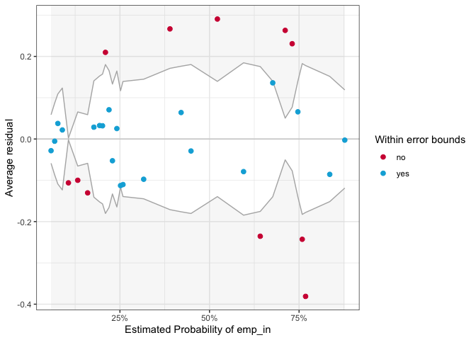Only 68% of the residuals are within the error bound, which (as happend in mod1) tells us that there is a problem in the model

We also check for heteroskedasticity with the Breush-Pagan test

mod2 <- glm(emp_in ~ educ + female + fin15 + age, 
            data=newdata2, family = "binomial")
library(lmtest)
bptest(mod2, data = newdata2, studentize = TRUE)

## 
##  studentized Breusch-Pagan test
## 
## data:  mod2
## BP = 52.811, df = 4, p-value = 9.332e-11

Our p value is < than 0.05. We have reject the null, and accept the fact that in our mod2 there is heteroskedasticity

We have to treat heteroskedascity and we cluster for the variable age

library(sandwich)
tab_model(mod2, vcov.fun = "CL", vcov.args = ~ age, show.obs = F, show.r2 = F, show.se = T, show.stat = T)

	Respondent is in the workforce
Predictors	Odds Ratios	std. Error	CI	Statistic	p
(Intercept)	1.72	0.64	0.49 – 6.05	0.85	0.397
Respondent education level	2.41	0.15	1.80 – 3.21	5.95	<0.001
Respondent is female: Female	0.12	0.17	0.08 – 0.16	-12.71	<0.001
fin15: no	0.33	0.35	0.16 – 0.65	-3.20	0.001
Respondent age	0.99	0.01	0.97 – 1.01	-1.28	0.200

As it happened in mod1, when we cluster by age the variable fin48 loses statistical significance. However, education keeps a very low p value, <0.001, and a coefficient of 2.44, meaning that the level of education increases the odds of being in the workforce. Being a woman also keeps a low p value, <0.001, with coefficient 0.12. Age in this case has a p value of 0.175, so it loses it statistical significance.

———————–MOD3———————————- In Model 3 we add the control variable “fin15” and “fin16”, which give us information about the conditions of the Jordanian labour market, and we keep all the other variables of mod1 and mod 2.

mod3 <- glm(emp_in ~ educ + female + fin15 + fin16 + fin48 + age ,
            data=newdata2, 
            family=binomial(link="logit"))
library(sjPlot)
tab_model(mod3)

	Respondent is in the workforce
Predictors	Odds Ratios	CI	p
(Intercept)	4.40	1.49 – 13.39	0.008
Respondent education level	2.23	1.70 – 2.93	<0.001
Respondent is female: Female	0.12	0.08 – 0.16	<0.001
fin15: no	0.38	0.20 – 0.71	0.003
fin16: no	0.48	0.29 – 0.79	0.004
fin48: no	0.54	0.31 – 0.95	0.036
Respondent age	0.98	0.97 – 0.99	0.001
Observations	975
R² Tjur	0.305

Interpretation: We see that all the variables have very small p values, but we suspect that there is heteroskedasticity in the model (given its similarity with mod 1 and mod2). We therefore run the test for multicollinearity and heteroskedasticity before interpreting the results.

—————-CHECKS MOD3————————————————– We can check for multicollinearity by constructing a plot:

library(performance)
plot(check_collinearity(mod3))

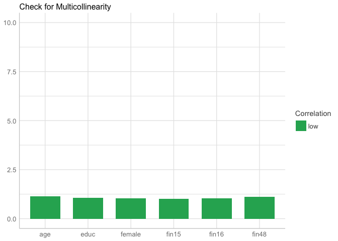we note that there is not collinerarity among the varibles We also check for heteroskedasticity with the Breush-Pagan test

mod3 <- glm(emp_in ~ educ + female + fin15 + fin16 + fin48 + age, 
            data=newdata2, family = "binomial")
library(lmtest)
bptest(mod3, data = newdata2, studentize = TRUE)

## 
##  studentized Breusch-Pagan test
## 
## data:  mod3
## BP = 50.364, df = 6, p-value = 3.974e-09

Our p value is < than 0.05. We have reject the null, and accept the fact that in our mod2 there is heteroskedasticity

We treat heteroskedascity as we did in the previous models, and we cluster for the variable age

library(sandwich)
tab_model(mod3, vcov.fun = "CL", vcov.args = ~ age, show.obs = F, show.r2 = F, show.se = T, show.stat = T)

	Respondent is in the workforce
Predictors	Odds Ratios	std. Error	CI	Statistic	p
(Intercept)	4.40	0.59	1.39 – 13.97	2.52	0.012
Respondent education level	2.23	0.14	1.68 – 2.95	5.57	<0.001
Respondent is female: Female	0.12	0.17	0.08 – 0.16	-13.06	<0.001
fin15: no	0.38	0.36	0.19 – 0.77	-2.70	0.007
fin16: no	0.48	0.26	0.28 – 0.79	-2.85	0.004
fin48: no	0.54	0.57	0.18 – 1.66	-1.07	0.285
Respondent age	0.98	0.01	0.97 – 1.00	-2.10	0.036

As it happened in mod1, when we cluster by age the variable fin48 loses statistical significance.Education keeps a very low p value, <0.001, and a coefficient of 2.20, meaning that the level of education increases the odds of being in the workforce. Being a woman also keeps a low p value, <0.001, with coefficient 0.12. Fin15 and fin16 both have low p values, 0.008 and 0.001 respectively, and they both indicate that not saving (either to start a business of for old age) decreases the odds of being in the workforce. Notably, in mod3 age has a p value of 0.014, and its coefficient indicates that the respondent’s age decreases the odds of being part of the workforce.

4. Results

——————–COMPARISON TO FIND THE BEST MODEL—————————- We now compare the performance of the models to see what is our best fit, by looking at their AIC. Given that we treated all models for heteroskedasticity in the same way, we can still compare their statistical power before the treatment

tab_model(mod3, mod2, mod1, show.loglik = T, show.aic = T, show.r2 = F)

	Respondent is in the workforce			Respondent is in the workforce			Respondent is in the workforce
Predictors	Odds Ratios	CI	p	Odds Ratios	CI	p	Odds Ratios	CI	p
(Intercept)	4.40	1.49 – 13.39	0.008	1.72	0.69 – 4.41	0.251	5.07	3.28 – 7.97	<0.001
Respondent education level	2.23	1.70 – 2.93	<0.001	2.41	1.85 – 3.14	<0.001
Respondent is female: Female	0.12	0.08 – 0.16	<0.001	0.12	0.08 – 0.16	<0.001	0.11	0.08 – 0.15	<0.001
fin15: no	0.38	0.20 – 0.71	0.003	0.33	0.17 – 0.60	<0.001
fin16: no	0.48	0.29 – 0.79	0.004
fin48: no	0.54	0.31 – 0.95	0.036				0.39	0.22 – 0.67	0.001
Respondent age	0.98	0.97 – 0.99	0.001	0.99	0.98 – 1.00	0.014	0.98	0.97 – 0.99	<0.001
Observations	975			983			990
AIC	995.955			1014.454			1070.948
log-Likelihood	-490.977			-502.227			-531.474

Mod3 has AIC of 994,951, Mod2 has a AIC of 1017.475 and mod1 has a AIC of 1075.186. Mod3 is therefore the best fit

We can also check using the Rock curve which is the best model betweem mod3 and mod2 (given that there isn’t a big difference between thier AIC)

library(plotROC)
test <- data.frame(resp = c(newdata2$emp_in), 
                    mod2 = predict(mod1, newdata2, type="response"),
                    mod3 = predict(mod2, newdata2, type="response"))
test <- melt_roc(test, "resp", c("mod2", "mod3"))
out <- ggplot(test, aes(d = D, m = M, colour = name)) +
   geom_roc(n.cuts = 0) + style_roc(theme = theme_grey)
out + annotate("text", x = .75, y = .25, label = paste(paste(unique(test$name), "AUC =", round(calc_auc(out)$AUC, 2)), collapse = "\n"))

## Warning in verify_d(data$d): D not labeled 0/1, assuming 1 = 0 and 2 = 1!

## Warning in verify_d(data$d): D not labeled 0/1, assuming 1 = 0 and 2 = 1!

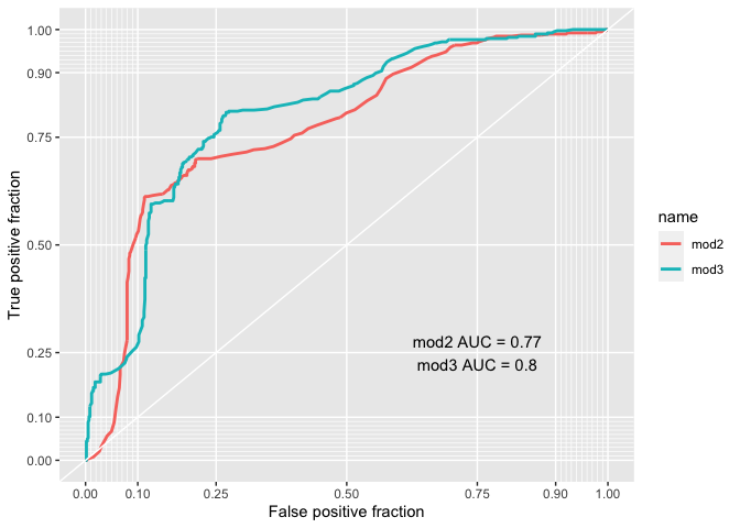
Mod3 has a bigger AUC (0.80) and it is therefore confirmed to be better.

5. Conclusion

What is the final interpretation that we can give to mod3, after having taken into consideration the heteroskedasticity issue?

library(sandwich)
tab_model(mod3, vcov.fun = "CL", vcov.args = ~ age, show.obs = F, show.r2 = F, show.se = T, show.stat = T)

	Respondent is in the workforce
Predictors	Odds Ratios	std. Error	CI	Statistic	p
(Intercept)	4.40	0.59	1.39 – 13.97	2.52	0.012
Respondent education level	2.23	0.14	1.68 – 2.95	5.57	<0.001
Respondent is female: Female	0.12	0.17	0.08 – 0.16	-13.06	<0.001
fin15: no	0.38	0.36	0.19 – 0.77	-2.70	0.007
fin16: no	0.48	0.26	0.28 – 0.79	-2.85	0.004
fin48: no	0.54	0.57	0.18 – 1.66	-1.07	0.285
Respondent age	0.98	0.01	0.97 – 1.00	-2.10	0.036

Final interpretation: We can conclude that, overall, it seems that our data doesn’t allow us to reject or accept the hypothesis that having a national ID increases or decreases the odds for individuals to be part of the workforce. In the context of the Jordanian labour market, the fact that it seems that this variable is not statistically significant, and therefore might be irrelevant in the “real world”, may be explained by the presence of a well-developed informal sector in the Jordanian labour market, where people can work with or without a national ID. This could be taken as evidence of the fact that individuals without a national ID should not be considered as “more advantaged” competitors to find employment in the informal market, against the allegation that undocumented forced migrants are “stealing” jobs from the Jordanians in the informal market. However, further research and better data are needed to explore in more detail this phenomenon. From our model 3 we can conclude that level of education is key to increase the odds of being in the workforce, and the checks for multicollinearity show that education level is not correlated with having a national ID. Being a woman is confirmed to be an obstacle in increasing one’s person odds of being in the workforce, with a very small coefficient (0.12). Age also appears negatively affecting the odds of being in the workforce, but by a higher coefficient (0.98). The variables indicating the possibility of the respondent to save to start a business (fin15) and for old age (fin16), help shading light on some characteristics of the labour-force of the Jordanian job market. From this analysis, we can deduce that individuals who do not have the possibility to save, either to start a business or for old age, have increased odds of being part of the workforce. If one considers the act of saving as a manifestation of a privileged economic status, it seems that the majority of the respondents that are part of the workforce in Jordan do not belong to this privileged group.

References:

Barbelet, Hagen-Zanker and Mansour-Ille, 2018, “the Jordan Compact: Lessons Learnt and implications for future refugee compacts”, ODI working paper Fallah, Kraff, Wahba, 2019, “The impact of refugees on employment and wages in Jordan”, Journal of Development Economics, 139